Alcohol and Aging (II)

I gave the book 3 stars on goodreads.

As is usual for publications of this nature, the book includes many chapters that cover similar topics and so the coverage can get a bit repetitive if you’re reading it from cover to cover the way I did; most of the various chapter authors obviously didn’t read the other contributions included in the book, and as each chapter is meant to stand on its own you end up with a lot of chapter introductions which cover very similar topics. If you can disregard such aspects it’s a decent book, which covers a wide variety of topics.

Below I have added some observations from some of the chapters of the book which I did not cover in my first post.

…

“It is widely accepted that consuming heavy amounts of alcohol and binge drinking are detrimental to the brain. Animal studies that have examined the anatomical changes that occur to the brain as a consequence of consuming alcohol indicate that heavy alcohol consumption and binge drinking leads to the death of existing neurons [10, 11] and prevents production of new neurons [12, 13]. […] While animal studies indicate that consuming even moderate amounts of alcohol is detrimental to the brain, the evidence from epidemiological studies is less clear. […] Epidemiological studies that have examined the relationship between late life alcohol consumption and cognition have frequently reported that older adults who consume light to moderate amounts of alcohol are less likely to develop dementia and have higher cognitive functioning compared to older adults who do not consume alcohol. […] In a meta-analysis of 15 prospective cohort studies, consuming light to moderate amounts of alcohol was associated with significantly lower relative risk (RR) for Alzheimer’s disease (RR=0.72, 95% CI=0.61–0.86), vascular dementia (RR=0.75, 95% CI=0.57–0.98), and any type of dementia (RR=0.74, 95% CI=0.61–0.91), but not cognitive decline (RR=0.28, 95 % CI=0.03–2.83) [31]. These findings are consistent with a previous meta-analysis by Peters et al. [33] in which light to moderate alcohol consumption was associated with a decreased risk for dementia (RR=0.63, 95 % CI=0.53–0.75) and Alzheimer’s disease (RR=0.57, 95 % CI=0.44–0.74), but not vascular dementia (RR=0.82, 95% CI=0.50–1.35) or cognitive decline RR=0.89, 95% CI=0.67–1.17). […] Mild cognitive impairment (MCI) has been used to describe the prodromal stage of Alzheimer’s disease […]. There is no strong evidence to suggest that consuming alcohol is protective against MCI [39, 40] and several studies have reported non-significant findings [41–43].”

“The majority of research on the relationship between alcohol consumption and cognitive outcomes has focused on the amount of alcohol consumed during old age, but there is a growing body of research that has examined the relationship between alcohol consumption during middle age and cognitive outcomes several years or decades later. The evidence from this area of research is mixed with some studies not detecting a significant relationship [17, 58, 59], while others have reported that light to moderate alcohol consumption is associated with preserved cognition [60] and decreased risk for cognitive impairment [31, 61, 62]. […] Several epidemiological studies have reported that light to moderate alcohol consumption is associated with a decreased risk for stroke, diabetes, and heart disease [36, 84, 85]. Similar to the U-shaped relationship between alcohol consumption and dementia, heavy alcohol consumption has been associated with poor health [86, 87]. The decreased risk for several metabolic and vascular health conditions for alcohol consumers has been attributed to antioxidants [54], greater concentrations of high-density lipoprotein cholesterol in the bloodstream [88], and reduced blood clot formation [89]. Stroke, diabetes, heart disease, and related conditions have all been associated with lower cognitive functioning during old age [90, 91]. The reduced prevalence of metabolic and vascular health conditions among light to moderate alcohol consumers may contribute to the decreased risk for dementia and cognitive decline for older adults who consume alcohol. A limitation of the hypothesis that the reduced risk for dementia among light and moderate alcohol consumers is conferred through the reduced prevalence of adverse health conditions associated with dementia is the possibility that this relationship is confounded by reverse causality. Alcohol consumption decreases with advancing age and adults may reduce their alcohol consumption in response to the onset of adverse health conditions […] the higher prevalence of dementia and lower cognitive functioning among abstainers may be due in part to their worse health rather than their alcohol consumption.”

“A limitation of large cohort studies is that subjects who choose not to participate or are unable to participate are often less healthy than those who do participate. Non-response bias becomes more pronounced with age because only subjects who have survived to old age and are healthy enough to participate are observed. Studies on alcohol consumption and cognition are sensitive to non-response bias because light and moderate drinkers who are not healthy enough to participate in the study will not be observed. Adults who survive to old age despite consuming very high amounts of alcohol represent an even more select segment of the general population because they may have genetic, behavioral, health, social, or other factors that protect them against the negative effects of heavy alcohol consumption. As a result, the analytic sample of epidemiological studies is more likely to be comprised of “healthy” drinkers, which biases results in favor of finding a positive effect of light to moderate alcohol consumption for cognition and health in general. […] The incidence of Alzheimer’s disease doubles every 5 years after 65 years of age [94] and nearly 40% of older adults aged 85 and over are diagnosed with Alzheimer’s disease [7]. The relatively old age of onset for most dementia cases means the observed protective effect of light to moderate alcohol consumption for dementia may be due to alcohol consumers being more likely to die or drop out of a study as a result of their alcohol consumption before they develop dementia. This bias may be especially strong for heavy alcohol consumers. Not properly accounting for death as a competing outcome has been observed to artificially increase the risk of dementia among older adults with diabetes [95] and the effect that death and other competing outcomes may have on the relationship between alcohol consumption and dementia risk is unclear. […] The majority of epidemiological studies that have studied the relationship between alcohol consumption and cognition treat abstainers as the reference category. This can be problematic because often times the abstainer or non-drinking category includes older adults who stopped consuming alcohol because of poor health […] Not differentiating former alcohol consumers from lifelong abstainers has been found to explain some but not all of the benefit of alcohol consumption for preventing mortality from cardiovascular causes [96].”

“It is common for people to engage in other behaviors while consuming alcohol. This complicates the relationship between alcohol consumption and cognition because many of the behaviors associated with alcohol consumption are positively and negatively associated with cognitive functioning. For example, alcohol consumers are more likely to smoke than non-drinkers [104] and smoking has been associated with an increased risk for dementia and cognitive decline [105]. […] The relationship between alcohol consumption and cognition may also differ between people with or without a history of mental illness. Depression reduces the volume of the hippocampus [106] and there is growing evidence that depression plays an important role in dementia. Depression during middle age is recognized as a risk factor for dementia [107], and high depressive symptoms during old age may be an early symptom of dementia [108]. Middle aged adults with depression or other mental illness who self-medicate with alcohol may be at especially high risk for dementia later in life because of synergistic effects that alcohol and depression has on the brain. […] While current evidence from epidemiological studies indicates that consuming light to moderate amounts of alcohol, in particular wine, does not negatively affect cognition and in many cases is associated with cognitive health, adults who do not consume alcohol should not be encouraged to increase their alcohol consumption until further research clarifies these relationships. Inconsistencies between studies on how alcohol consumption categories are defined make it difficult to determine the “optimal” amount of alcohol consumption to prevent dementia. It is likely that the optimal amount of alcohol varies according to a person’s gender, as well as genetic, physiological, behavioral, and health characteristics, making the issue extremely complex.”

“Falls are the leading cause of both fatal and nonfatal injuries among older adults, with one in three older adults falling each year, and 20–30% of people who fall suffer moderate to severe injuries such as lacerations, hip fractures, and head traumas. In fact, falls are the foremost cause of both fractures and traumatic brain injury (TBI) among older adults […] In 2013, 2.5 million nonfatal falls among older adults were treated in ED and more than 734,000 of these patients were hospitalized. […] Our analysis of the 2012 Nationwide Emergency Department Sample (NEDS) data set show that fall-related injury was a presenting problem among 12% of all ED visits by those aged 65+, with significant differences among age groups: 9% among the 65–74 age group, 12 % among the 75–84 age group, and 18 % among the 85+ age group [4]. […] heavy alcohol use predicts fractures. For example, among those 55+ years old in a health survey in England, men who consumed more than 8 units of alcohol and women who consumed more than 6 units on their heaviest drinking day in the past week had significantly increased odds of fractures (OR =1.65, 95% CI =1.37–1.98 for men and OR=2.07, 95% CI =1.28–3.35 for women) [63]. […] The 2008–2009 Canadian Community Health Survey-Healthy Aging also showed that consumption of at least one alcoholic drink per week increased the odds of falling by 40 % among those 65+ years [57].”

…

I at first was not much impressed by the effect sizes mentioned above because there are surely 100 relevant variables they didn’t account for/couldn’t account for, but then I thought a bit more about it. An important observation here – they don’t mention it in the coverage, but it sprang to mind – is that if sick or frail elderly people consume less alcohol than their more healthy counterparts, and are more likely to not consume alcohol (which they do, and which they are, we know this), and if frail or sick(er) elderly people are more likely to suffer a fall/fracture than are people who are relatively healthy (they are, again, we know this), well, then you’d expect consumption of alcohol to be found to have a ‘protective effect’ simply due to confounding by (reverse) indication (unless the researchers were really careful about adjusting for such things, but no such adjustments are mentioned in the coverage, which makes sense as these are just raw numbers being reported). The point is that the null here should not be that ‘these groups should be expected to have the same fall rate/fracture rate’, but rather ‘people who drink alcohol should be expected to be doing better, all else equal’ – but they aren’t, quite the reverse. So ‘the true effect size’ here may be larger than what you’d think.

I’m reasonably sure things are a lot more complicated than the above makes it appear (because of those 100 relevant variables we were talking about…), but I find it interesting anyway. Two more things to note: 1. Have another look at the numbers above if they didn’t sink in the first time. This is more than 10% of emergency department visits for that age group. Falls are a really big deal. 2. Fractures in the elderly are also a potentially really big deal. Here’s a sample quote: “One-fifth of hip fracture victims will die within 6 months of the injury, and only 50% will return to their previous level of independence.” (link). In some contexts, a fall is worse news than a cancer diagnosis, and they are very common events in the elderly. This also means that even relatively small effect sizes here can translate into quite large public health effects, because baseline incidence is so high.

…

“The older adult population is a disproportionate consumer of prescription and over-the-counter medications. In a nationally representative sample of community-dwelling adults aged 57–84 years from the National Social Life, Health, and Aging Project (NSHAP) in 2005–2006, 81 % regularly used at least one prescription medication on a regular basis and 29% used at least five prescription medications. Forty-two percent used at least one nonprescription medication and concurrent use with a prescription medication was common, with 46% of prescription medication users also using OTC medications [2]. Prescription drug use by older adults in the U.S. is also growing. The percentage of older adults taking at least one prescription drug in the last 30 days increased from 73.6% in 1988–1994 to 89.7 % in 2007–2010 and the percentage taking five or more prescription drugs in the last 30 days increased from 13.8% in 1988–1994 to 39.7 % in 2007–2010 [3].”

“The aging process can affect the response to a medication by altering its pharmacokinetics and pharmacodynamics [9, 10]. Reduced gastrointestinal motility and gastric acidity can alter the rate or extent of drug absorption. Changes in body composition, including decreased total body water and increased body fat can alter drug distribution. For alcohol, changes in body composition result in higher blood alcohol levels in older adults compared to younger adults after the same dose or quantity  of alcohol consumed. Decreased size of the liver, hepatic blood flow, and function of Phase I (oxidation, reduction, and hydrolysis) metabolic pathways result in reduced drug metabolism and increased drug exposure for drugs that undergo Phase I metabolism. Phase II hepatic metabolic pathways are generally preserved with aging. Decreased size of the kidney, renal blood flow, and glomerular filtration result in slower elimination of medications and metabolites by the kidney and increased drug exposure for medications that undergo renal elimination. Age-related impairment of homeostatic mechanisms and changes in receptor number and function can result in changes in pharmacodynamics as well. Older adults are generally more sensitive to the effects of medications and alcohol which act on the central nervous system for example. The consequences of these physiologic changes with aging are that older adults often experience increased drug exposure for the same dose (higher drug concentrations over time) and increased sensitivity to medications (greater response at a given drug concentration) than their younger counterparts.”

“Aging-related changes in physiology are not the only sources of variability in pharmacokinetics and pharmacodynamics that must be considered for an individual person. Older adults experience more chronic diseases that may decrease drug metabolism and renal elimination than younger cohorts. Frailty may result in further decline in drug metabolism, including Phase II metabolic pathways in the liver […] Drug interactions must also be considered […] A drug interaction is defined as a clinically meaningful change in the effect of one drug when coadministered with another drug [12]. Many drugs, including alcohol, have the potential for a drug interaction when administered concurrently, but whether a clinically meaningful change in effect occurs for a specific person depends on patient-specifc factors including age. Drug interactions are generally classified as pharmacokinetic interactions, where one drug alters the absorption, distribution, metabolism, or elimination of another drug resulting in increased or decreased drug exposure, or pharmacodynamic interactions, where one drug alters the response to another medication through additive or antagonistic pharmacologic effects [13]. An adverse drug event occurs when a pharmacokinetic or pharmacodynamic interaction or combination of both results in changes in drug exposure or response that lead to negative clinical outcomes. The adverse drug event could be a therapeutic failure if drug exposure is decreased or the pharmacologic response is antagonistic. The adverse drug event could be drug toxicity if the drug exposure is increased or the pharmacologic response is additive or synergistic. The threshold for experiencing an adverse event is often lower in older adults due to physiologic changes with aging and medical comorbidities, increasing their risk of experiencing an adverse drug event when medications are taken concurrently.”

“A large number of potential medication–alcohol interactions have been reported in the literature. Mechanisms of these interactions range from pharmacokinetic interactions affecting either alcohol or medication exposure to pharmacodynamics interactions resulting in exaggerated response. […] Epidemiologic evidence suggests that concurrent use of alcohol and medications among older adults is common. […] In a nationally representative U.S. sample of community-dwelling older adults in the National Social Life, Health and Aging Project (NSHAP) 2005–2006, 41% of participants reported consuming alcohol at least once per week and 20% were at risk for an alcohol–medication interaction because they were using both alcohol and alcohol-interacting medications on a regular basis [17]. […] Among participants in the Pennsylvania Assistance Contract for the Elderly program (aged 65–106 years) taking at least one prescription medication, 77% were taking an alcohol-interacting medication and 19% of the alcohol-interacting medication users reported concurrent use of alcohol [18]. […] Although these studies do not document adverse outcomes associated with alcohol–medication interactions, they do document that the potential exists for many older adults. […] High prevalence of concurrent use of alcohol and alcohol-interacting medications have also been reported in Australian men (43% of sedative or anxiolytic users were daily drinkers) [19], in older adults in Finland (42% of at-risk alcohol users were also taking alcohol-interacting medications) [20], and in older Irish adults (72% of participants were exposed to alcohol-interacting medications and 60% of these reported concurrent alcohol use) [21]. Drinking and medication use patterns in older adults may differ across countries, but alcohol–medication interactions appear to be a worldwide concern. […] Polypharmacy in general, and psychotropic burden specifically, has been associated with an increased risk of experiencing a geriatric syndrome such as falls or delirium, in older adults [26, 27]. Based on its pharmacology, alcohol can be considered as a psychotropic drug, and alcohol use should be assessed as part of the medication regimen evaluation to support efforts to prevent or manage geriatric syndromes. […] Combining alcohol and CNS active medications can be particularly problematic […] Older adults suffering from sleep problems or pain may be a particular risk for alcohol–medication interaction-related adverse events.”

“In general, alcohol use in younger couples has been found to be highly concordant, that is, individuals in a relationship tend to engage in similar drinking behaviors [67,68]. Less is known, however, about alcohol use concordance between older couples. Graham and Braun [69] examined similarities in drinking behavior between spouses in a study of 826 community-dwelling older adults in Ontario, Canada. Results showed high concordance of drinking between spouses — whether they drank at all, how much they drank, and how frequently. […] Social learning theory suggests that alcohol use trajectories are strongly influenced by attitudes and behaviors of an individual’s social networks, particularly family and friends. When individuals engage in social activities with family and friends who approve of and engage in drinking, alcohol use, and misuse are reinforced [58, 59]. Evidence shows that among older adults, participation in social activities is correlated with higher levels of alcohol consumption [34, 60]. […] Brennan and Moos [29] […] found that older adults who reported less empathy and support from friends drank more alcohol, were more depressed, and were less self-confident. More stressors involving friends were associated with more drinking problems. Similar to the findings on marital conflict […], conflict in close friendships can prompt alcohol-use problems; conversely, these relationships can suffer as a result of alcohol-related problems. […] As opposed to social network theory […], social selection theory proposes that alcohol consumption changes an individual’s social context [33]. Studies among younger adults have shown that heavier drinkers chose partners and friends who approve of heavier drinking [70] and that excessive drinking can alienate social networks. The Moos study supports the idea that social selection also has a strong influence on drinking behavior among older adults.”

“Traditionally, treatment studies in addiction have excluded patients over the age of 65. This bias has left a tremendous gap in knowledge regarding treatment outcomes and an understanding of the neurobiology of addiction in older adults.”

“Alcohol use causes well-established changes in sleep patterns, such as decreased sleep latency, decreased stage IV sleep, and precipitation or aggravation of sleep apnea [101]. There are also age-associated changes in sleep patterns including increased REM episodes, a decrease in REM length, a decrease in stage III and IV sleep, and increased awakenings. Age-associated changes in sleep can all be worsened by alcohol use and depression. Moeller and colleagues [102] demonstrated in younger subjects that alcohol and depression had additive effects upon sleep disturbances when they occurred together [102]. Wagman and colleagues [101] also have demonstrated that abstinent alcoholics did not sleep well because of insomnia, frequent awakenings, and REM fragmentation [101]; however, when these subjects ingested alcohol, sleep periodicity normalized and REM sleep was temporarily suppressed, suggesting that alcohol use could be used to self-medicate for sleep disturbances. A common anecdote from patients is that alcohol is used to help with sleep problems. […] The use of alcohol to self-medicate is considered maladaptive [34] and is associated with a host of negative outcomes. […] The use of alcohol to aid with sleep has been found to disrupt sleep architecture and cause sleep-related problems and daytime sleepiness [35, 36, 46]. Though alcohol is commonly used to aid with sleep initiation, it can worsen sleep-related breathing disorders and cause snoring and obstructive sleep apnea [36].”

“Epidemiologic studies have clearly demonstrated that comorbidity between alcohol use and other psychiatric symptoms is common in younger age groups. Less is known about comorbidity between alcohol use and psychiatric illness in late life [88]. […] Blow et al. [90] reviewed the diagnosis of 3,986 VA patients between ages 60 and 69 presenting for alcohol treatment [90]. The most common comorbid psychiatric disorder was an affective disorder found in 21 % of the patients. […] Blazer et al. [91] studied 997 community dwelling elderly of whom only 4.5% had a history of alcohol use problems [91]; […] of these subjects, almost half had a comorbid diagnosis of depression or dysthymia. Comorbid depressive symptoms are not only common in late life but are also an important factor in the course and prognosis of psychiatric disorders. Depressed alcoholics have been shown to have a more complicated clinical course of depression with an increased risk of suicide and more social dysfunction than non-depressed alcoholics [92–96]. […]  Alcohol use prior to late life has also been shown to influence treatment of late life depression. Cook and colleagues [94] found that a prior history of alcohol use problems predicted a more severe and chronic course for depression [94]. […] The effect of past heavy alcohol use is [also] highlighted in the findings from the Liverpool Longitudinal Study demonstrating a fivefold increase in psychiatric illness among elderly men who had a lifetime history of 5 or more years of heavy drinking [24]. The association between heavy alcohol consumption in earlier years and psychiatric morbidity in later life was not explained by current drinking habits. […] While Wernicke-Korsakoff’s syndrome is well described and often caused by alcohol use disorders, alcohol-related dementia may be difficult to differentiate from Alzheimer’s disease. Clinical diagnostic criteria for alcohol-related dementia (ARD) have been proposed and now validated in at least one trial, suggesting a method for distinguishing ARD, including Wernicke-Korsakoff’s syndrome, from other types of dementia [97, 98]. […] Finlayson et al. [100] found that 49 of 216 (23%) elderly patients presenting for alcohol treatment had dementia associated with alcohol use disorders [100].”

 

Occupational Epidemiology (II)

Some more observations from the book below.

…

“RD [Retinal detachment] is the separation of the neurosensory retina from the underlying retinal pigment epithelium.¹ RD is often preceded by posterior vitreous detachment — the separation of the posterior vitreous from the retina as a result of vitreous degeneration and shrinkage² — which gives rise to the sudden appearance of floaters and flashes. Late symptoms of RD may include visual field defects (shadows, curtains) or even blindness. The success rate of RD surgery has been reported to be over 90%;³ however, a loss of visual acuity is frequently reported by patients, particularly if the macula is involved.⁴ Since the natural history of RD can be influenced by early diagnosis, patients experiencing symptoms of posterior vitreous detachment are advised to undergo an ophthalmic examination.⁵ […] Studies of the incidence of RD give estimates ranging from 6.3 to 17.9 cases per 100 000 person-years.⁶ […] Age is a well-known risk factor for RD. In most studies the peak incidence was recorded among subjects in their seventh decade of life. A secondary peak at a younger age (20–30 years) has been identified […] attributed to RD among highly myopic patients.⁶ Indeed, depending on the severity,
myopia is associated with a four- to ten-fold increase in risk of RD.⁷ [Diabetics with retinopathy are also at increased risk of RD, US] […] While secondary prevention of RD is current practice, no effective primary prevention strategy is available at present. The idea is widespread among practitioners that RD is not preventable, probably the consequence of our historically poor understanding of the aetiology of RD. For instance, on the website of the Mayo Clinic — one of the top-ranked hospitals for ophthalmology in the US — it is possible to read that ‘There’s no way to prevent retinal detachment’.⁹”

“Intraocular pressure […] is influenced by physical activity. Dynamic exercise causes an acute reduction in intraocular pressure, whereas physical fitness is associated with a lower baseline value.²⁹ Conversely, a sudden rise in intraocular pressure has been reported during the Valsalva manoeuvre.^30-32 […] Occupational physical activity may […] cause both short- and long-term variations in intraocular pressure. On the one hand, physically demanding jobs may contribute to decreased baseline levels by increasing physical fitness but, on the other hand, lifting tasks may cause an important acute increase in pressure. Moreover, the eye of a manual worker who performs repeated lifting tasks involving the Valsalva manoeuvre may undergo several dramatic changes in intraocular pressure within a single working shift. […] A case-control study was carried out to test the hypothesis that repeated lifting tasks involving the Valsalva manoeuvre could be a risk factor for RD. […] heavy lifting was a strong risk factor for RD (OR 4.4, 95% CI 1.6–13). Intriguingly, body mass index (BMI) also showed a clear association with RD (top quartile: OR 6.8, 95% CI 1.6–29). […] Based on their findings, the authors concluded that heavy occupational lifting (involving the Valsalva manoeuvre) may be a relevant risk factor for RD in myopics.”

“The proportion of the world’s population over 60 is forecast to double from 11.6% in 2012 to 21.8% in 2050.¹ […] the International Labour Organization notes that, worldwide, just 40% of the working age population has legal pension coverage, and only 26% of the working population is effectively covered by old-age pension schemes. […] in less developed regions, labour force participation in those over 65 is much higher than in more developed regions.⁸ […] Longer working lives increase cumulative exposures, as well as increasing the time since exposure — important when there is a long latency period between exposure and resultant disease. Further, some exposures may have a greater effect when they occur to older workers, e.g. carcinogens that are promoters rather than initiators. […] Older workers tend to have more chronic health conditions. […] Older workers have fewer injuries, but take longer to recover. […] For some ‘knowledge workers’, like physicians, even a relatively minor cognitive decline […] might compromise their competence. […]  Most past studies have treated age as merely a confounding variable and rarely, if ever, have considered it an effect modifier. […]  Jex and colleagues²⁴ argue that conceptually we should treat age as the variable of interest so that other variables are viewed as moderating the impact of age. […] The single best improvement to epidemiological research on ageing workers is to conduct longitudinal studies, including follow-up of workers into retirement. Cross-sectional designs almost certainly incur the healthy survivor effect, since unhealthy workers may retire early.²⁵ […] Analyses should distinguish ageing per se, genetic factors, work exposures, and lifestyle in order to understand their relative and combined effects on health.”

“Musculoskeletal disorders have long been recognized as an important source of morbidity and disability in many occupational populations.^1,2 Most musculoskeletal disorders, for most people, are characterized by recurrent episodes of pain that vary in severity and in their consequences for work. Most episodes subside uneventfully within days or weeks, often without any intervention, though about half of people continue to experience some pain and functional limitations after 12 months.^3,4 In working populations, musculoskeletal disorders may lead to a spell of sickness absence. Sickness absence is increasingly used as a health parameter of interest when studying the consequences of functional limitations due to disease in occupational groups. Since duration of sickness absence contributes substantially to the indirect costs of illness, interventions increasingly address return to work (RTW).⁵ […] The Clinical Standards Advisory Group in the United Kingdom reported RTW within 2 weeks for 75% of all low back pain (LBP) absence episodes and suggested that approximately 50% of all work days lost due to back pain in the working population are from the 85% of people who are off work for less than 7 days.^6″

“Any RTW curve over time can be described with a mathematical Weibull function.¹⁵ This Weibull function is characterized by a scale parameter λ and a shape parameter k. The scale parameter λ is a function of different covariates that include the intervention effect, preferably expressed as hazard ratio (HR) between the intervention group and the reference group in a Cox’s proportional hazards regression model. The shape parameter k reflects the relative increase or decrease in survival time, thus expressing how much the RTW rate will decrease with prolonged sick leave. […] a HR as measure of effect can be introduced as a covariate in the scale parameter λ in the Weibull model and the difference in areas under the curve between the intervention model and the basic model will give the improvement in sickness absence days due to the intervention. By introducing different times of starting the intervention among those workers still on sick leave, the impact of timing of enrolment can be evaluated. Subsequently, the estimated changes in total sickness absence days can be expressed in a benefit/cost ratio (BC ratio), where benefits are the costs saved due to a reduction in sickness absence and costs are the expenditures relating to the intervention.^15″

“A crucial factor in understanding why interventions are effective or not is the timing of the enrolment of workers on sick leave into the intervention. The RTW pattern over time […] has important consequences for appropriate timing of the best window for effective clinical and occupational interventions. The evidence presented by Palmer and colleagues clearly suggests that [in the context of LBP] a stepped care approach is required. In the first step of rapid RTW, most workers will return to work even without specific interventions. Simple, short interventions involving effective coordination and cooperation between primary health care and the workplace will be sufficient to help the majority of workers to achieve an early RTW. In the second step, more expensive, structured interventions are reserved for those who are having difficulties returning, typically between 4 weeks and 3 months. However, to date there is little evidence on the optimal timing of such interventions for workers on sick leave due to LBP.^14,15 […] the cost-benefits of a structured RTW intervention among workers on sick leave will be determined by the effectiveness of the intervention, the natural speed of RTW in the target population, the timing of the enrolment of workers into the intervention, and the costs of both the intervention and of a day of sickness absence. […] The cost-effectiveness of a RTW intervention will be determined by the effectiveness of the intervention, the costs of the intervention and of a day of sickness absence, the natural course of RTW in the target population, the timing of the enrolment of workers into the RTW intervention, and the time lag before the intervention takes effect. The latter three factors are seldom taken into consideration in systematic reviews and guidelines for management of RTW, although their impact may easily be as important  as classical measures of effectiveness, such as effect size or HR.”

“In order to obtain information of the highest quality and utility, surveillance schemes have to be designed, set up, and managed with the same methodological rigour as high-calibre prospective cohort studies. Whether surveillance schemes are voluntary or not, considerable effort has to be invested to ensure a satisfactory and sufficient denominator, the best numerator quality, and the most complete ascertainment. Although the force of statute is relied upon in some surveillance schemes, even in these the initial and continuing motivation of the reporters (usually physicians) is paramount. […] There is a surveillance ‘pyramid’ within which the patient’s own perception is at the base, the GP is at a higher level, and the clinical specialist is close to the apex. The source of the surveillance reports affects the numerator because case severity and case mix differ according to the level in the pyramid.¹⁹ Although incidence rate estimates may be expected to be lower at the higher levels in the surveillance pyramid this is not necessarily always the case. […] Although surveillance undertaken by physicians who specialize in the organ system concerned or in occupational disease (or in both aspects) may be considered to be the medical ‘gold standard’ it can suffer from a more limited patient catchment because of various referral filters. Surveillance by GPs will capture numerator cases as close to the base of the pyramid as possible, but may suffer from greater diagnostic variation than surveillance by specialists. Limiting recruitment to GPs with a special interest, and some training, in occupational medicine is a compromise between the two levels.²⁰”

“When surveillance is part of a statutory or other compulsory scheme then incident case identification is a continuous and ongoing process. However, when surveillance is voluntary, for a research objective, it may be preferable to sample over shorter, randomly selected intervals, so as to reduce the demands associated with the data collection and ‘reporting fatigue’. Evidence so far suggests that sampling over shorter time intervals results in higher incidence estimates than continuous sampling.²¹ […] Although reporting fatigue is an important consideration in tempering conclusions drawn from […] multilevel models, it is possible to take account of this potential bias in various ways. For example, when evaluating interventions, temporal trends in outcomes resulting from other exposures can be used to control for fatigue.^23,24 The phenomenon of reporting fatigue may be characterized by an ‘excess of zeroes’ beyond what is expected of a Poisson distribution and this effect can be quantified.²⁷ […] There are several considerations in determining incidence from surveillance data. It is possible to calculate an incidence rate based on the general population, on the population of working age, or on the total working population,19 since these denominator bases are generally readily available, but such rates are not the most useful in determining risk. Therefore, incidence rates are usually calculated in respect of specific occupations or industries.²² […] Ideally, incidence rates should be expressed in relation to quantitative estimates of exposure but most surveillance schemes would require additional data collection as special exercises to achieve this aim.” [for much more on these topics, see also M’ikanatha & Iskander’s book.]

“Estimates of lung cancer risk attributable to occupational exposures vary considerably by geographical area and depend on study design, especially on the exposure assessment method, but may account for around 5–20% of cancers among men, but less (<5%) among women;² among workers exposed to (suspected) lung carcinogens, the percentage will be higher. […] most exposure to known lung carcinogens originates from occupational settings and will affect millions of workers worldwide.  Although it has been established that these agents are carcinogenic, only limited evidence is available about the risks encountered at much lower levels in the general population. […] One of the major challenges in community-based occupational epidemiological studies has been valid assessment of the occupational exposures experienced by the population at large. Contrary to the detailed information usually available for an industrial population (e.g. in a retrospective cohort study in a large chemical company) that often allows for quantitative exposure estimation, community-based studies […] have to rely on less precise and less valid estimates. The choice of method of exposure assessment to be applied in an epidemiological study depends on the study design, but it boils down to choosing between acquiring self-reported exposure, expert-based individual exposure assessment, or linking self-reported job histories with job-exposure matrices (JEMs) developed by experts. […] JEMs have been around for more than three decades.¹⁴ Their main distinction from either self-reported or expert-based exposure assessment methods is that exposures are no longer assigned at the individual subject level but at job or task level. As a result, JEMs make no distinction in assigned exposure between individuals performing the same job, or even between individuals performing a similar job in different companies. […] With the great majority of occupational exposures having a rather low prevalence (<10%) in the general population it is […] extremely important that JEMs are developed aiming at a highly specific exposure assessment so that only jobs with a high likelihood (prevalence) and intensity of exposure are considered to be exposed. Aiming at a high sensitivity would be disastrous because a high sensitivity would lead to an enormous number of individuals being assigned an exposure while actually being unexposed […] Combinations of the methods just described exist as well”.

“Community-based studies, by definition, address a wider range of types of exposure and a much wider range of encountered exposure levels (e.g. relatively high exposures in primary production but often lower in downstream use, or among indirectly exposed individuals). A limitation of single community-based studies is often the relatively low number of exposed individuals. Pooling across studies might therefore be beneficial. […] Pooling projects need careful planning and coordination, because the original studies were conducted for different purposes, at different time periods, using different questionnaires. This heterogeneity is sometimes perceived as a disadvantage but also implies variations that can be studied and thereby provide important insights. Every pooling project has its own dynamics but there are several general challenges that most pooling projects confront. Creating common variables for all studies can stretch from simple re-naming of variables […] or recoding of units […] to the re-categorization of national educational systems […] into years of formal education. Another challenge is to harmonize the different classification systems of, for example, diseases (e.g. International Classification of Disease (ICD)-9 versus ICD-10), occupations […], and industries […]. This requires experts in these respective fields as well as considerable time and money. Harmonization of data may mean losing some information; for example, ISCO-68 contains more detail than ISCO-88, which makes it possible to recode ISCO-68 to ISCO-88 with only a little loss of detail, but it is not possible to recode ISCO-88 to ISCO-68 without losing one or two digits in the job code. […] Making the most of the data may imply that not all studies will qualify for all analyses. For example, if a study did not collect data regarding lung cancer cell type, it can contribute to the overall analyses but not to the cell type-specific analyses. It is important to remember that the quality of the original data is critical; poor data do not become better by pooling.”

Biodemography of aging (IV)

My working assumption as I was reading part two of the book was that I would not be covering that part of the book in much detail here because it would simply be too much work to make such posts legible to the readership of this blog. However I then later, while writing this post, had the thought that given that almost nobody reads along here anyway (I’m not complaining, mind you – this is how I like it these days), the main beneficiary of my blog posts will always be myself, which lead to the related observation/notion that I should not be limiting my coverage of interesting stuff here simply because some hypothetical and probably nonexistent readership out there might not be able to follow the coverage. So when I started out writing this post I was working under the assumption that it would be my last post about the book, but I now feel sure that if I find the time I’ll add at least one more post about the book’s statistics coverage. On a related note I am explicitly making the observation here that this post was written for my benefit, not yours. You can read it if you like, or not, but it was not really written for you.

I have added bold a few places to emphasize key concepts and observations from the quoted paragraphs and in order to make the post easier for me to navigate later (all the italics below are on the other hand those of the authors of the book).

…

“Biodemography is a multidisciplinary branch of science that unites under its umbrella various analytic approaches aimed at integrating biological knowledge and methods and traditional demographic analyses to shed more light on variability in mortality and health across populations and between individuals. Biodemography of aging is a special subfield of biodemography that focuses on understanding the impact of processes related to aging on health and longevity.”

“Mortality rates as a function of age are a cornerstone of many demographic analyses. The longitudinal age trajectories of biomarkers add a new dimension to the traditional demographic analyses: the mortality rate becomes a function of not only age but also of these biomarkers (with additional dependence on a set of sociodemographic variables). Such analyses should incorporate dynamic characteristics of trajectories of biomarkers to evaluate their impact on mortality or other outcomes of interest. Traditional analyses using baseline values of biomarkers (e.g., Cox proportional hazards or logistic regression models) do not take into account these dynamics. One approach to the evaluation of the impact of biomarkers on mortality rates is to use the Cox proportional hazards model with time-dependent covariates; this approach is used extensively in various applications and is available in all popular statistical packages. In such a model, the biomarker is considered a time-dependent covariate of the hazard rate and the corresponding regression parameter is estimated along with standard errors to make statistical inference on the direction and the significance of the effect of the biomarker on the outcome of interest (e.g., mortality). However, the choice of the analytic approach should not be governed exclusively by its simplicity or convenience of application. It is essential to consider whether the method gives meaningful and interpretable results relevant to the research agenda. In the particular case of biodemographic analyses, the Cox proportional hazards model with time-dependent covariates is not the best choice.”

“Longitudinal studies of aging present special methodological challenges due to inherent characteristics of the data that need to be addressed in order to avoid biased inference. The challenges are related to the fact that the populations under study (aging individuals) experience substantial dropout rates related to death or poor health and often have co-morbid conditions related to the disease of interest. The standard assumption made in longitudinal analyses (although usually not explicitly mentioned in publications) is that dropout (e.g., death) is not associated with the outcome of interest. While this can be safely assumed in many general longitudinal studies (where, e.g., the main causes of dropout might be the administrative end of the study or moving out of the study area, which are presumably not related to the studied outcomes), the very nature of the longitudinal outcomes (e.g., measurements of some physiological biomarkers) analyzed in a longitudinal study of aging assumes that they are (at least hypothetically) related to the process of aging. Because the process of aging leads to the development of diseases and, eventually, death, in longitudinal studies of aging an assumption of non-association of the reason for dropout and the outcome of interest is, at best, risky, and usually is wrong. As an illustration, we found that the average trajectories of different physiological indices of individuals dying at earlier ages markedly deviate from those of long-lived individuals, both in the entire Framingham original cohort […] and also among carriers of specific alleles […] In such a situation, panel compositional changes due to attrition affect the averaging procedure and modify the averages in the total sample. Furthermore, biomarkers are subject to measurement error and random biological variability. They are usually collected intermittently at examination times which may be sparse and typically biomarkers are not observed at event times. It is well known in the statistical literature that ignoring measurement errors and biological variation in such variables and using their observed “raw” values as time-dependent covariates in a Cox regression model may lead to biased estimates and incorrect inferences […] Standard methods of survival analysis such as the Cox proportional hazards model (Cox 1972) with time-dependent covariates should be avoided in analyses of biomarkers measured with errors because they can lead to biased estimates.”

“Statistical methods aimed at analyses of time-to-event data jointly with longitudinal measurements have become known in the mainstream biostatistical literature as “joint models for longitudinal and time-to-event data” (“survival” or “failure time” are often used interchangeably with “time-to-event”) or simply “joint models.” This is an active and fruitful area of biostatistics with an explosive growth in recent years. […] The standard joint model consists of two parts, the first representing the dynamics of longitudinal data (which is referred to as the “longitudinal sub-model”) and the second one modeling survival or, generally, time-to-event data (which is referred to as the “survival sub-model”). […] Numerous extensions of this basic model have appeared in the joint modeling literature in recent decades, providing great flexibility in applications to a wide range of practical problems. […] The standard parameterization of the joint model (11.2) assumes that the risk of the event at age t depends on the current “true” value of the longitudinal biomarker at this age. While this is a reasonable assumption in general, it may be argued that additional dynamic characteristics of the longitudinal trajectory can also play a role in the risk of death or onset of a disease. For example, if two individuals at the same age have exactly the same level of some biomarker at this age, but the trajectory for the first individual increases faster with age than that of the second one, then the first individual can have worse survival chances for subsequent years. […] Therefore, extensions of the basic parameterization of joint models allowing for dependence of the risk of an event on such dynamic characteristics of the longitudinal trajectory can provide additional opportunities for comprehensive analyses of relationships between the risks and longitudinal trajectories. Several authors have considered such extended models. […] joint models are computationally intensive and are sometimes prone to convergence problems [however such] models provide more efficient estimates of the effect of a covariate […] on the time-to-event outcome in the case in which there is […] an effect of the covariate on the longitudinal trajectory of a biomarker. This means that analyses of longitudinal and time-to-event data in joint models may require smaller sample sizes to achieve comparable statistical power with analyses based on time-to-event data alone (Chen et al. 2011).”

“To be useful as a tool for biodemographers and gerontologists who seek biological explanations for observed processes, models of longitudinal data should be based on realistic assumptions and reflect relevant knowledge accumulated in the field. An example is the shape of the risk functions. Epidemiological studies show that the conditional hazards of health and survival events considered as functions of risk factors often have U- or J-shapes […], so a model of aging-related changes should incorporate this information. In addition, risk variables, and, what is very important, their effects on the risks of corresponding health and survival events, experience aging-related changes and these can differ among individuals. […] An important class of models for joint analyses of longitudinal and time-to-event data incorporating a stochastic process for description of longitudinal measurements uses an epidemiologically-justified assumption of a quadratic hazard (i.e., U-shaped in general and J-shaped for variables that can take values only on one side of the U-curve) considered as a function of physiological variables. Quadratic hazard models have been developed and intensively applied in studies of human longitudinal data”.

“Various approaches to statistical model building and data analysis that incorporate unobserved heterogeneity are ubiquitous in different scientific disciplines. Unobserved heterogeneity in models of health and survival outcomes can arise because there may be relevant risk factors affecting an outcome of interest that are either unknown or not measured in the data. Frailty models introduce the concept of unobserved heterogeneity in survival analysis for time-to-event data. […] Individual age trajectories of biomarkers can differ due to various observed as well as unobserved (and unknown) factors and such individual differences propagate to differences in risks of related time-to-event outcomes such as the onset of a disease or death. […] The joint analysis of longitudinal and time-to-event data is the realm of a special area of biostatistics named “joint models for longitudinal and time-to-event data” or simply “joint models” […] Approaches that incorporate heterogeneity in populations through random variables with continuous distributions (as in the standard joint models and their extensions […]) assume that the risks of events and longitudinal trajectories follow similar patterns for all individuals in a population (e.g., that biomarkers change linearly with age for all individuals). Although such homogeneity in patterns can be justifiable for some applications, generally this is a rather strict assumption […] A population under study may consist of subpopulations with distinct patterns of longitudinal trajectories of biomarkers that can also have different effects on the time-to-event outcome in each subpopulation. When such subpopulations can be defined on the base of observed covariate(s), one can perform stratified analyses applying different models for each subpopulation. However, observed covariates may not capture the entire heterogeneity in the population in which case it may be useful to conceive of the population as consisting of latent subpopulations defined by unobserved characteristics. Special methodological approaches are necessary to accommodate such hidden heterogeneity. Within the joint modeling framework, a special class of models, joint latent class models, was developed to account for such heterogeneity […] The joint latent class model has three components. First, it is assumed that a population consists of a fixed number of (latent) subpopulations. The latent class indicator represents the latent class membership and the probability of belonging to the latent class is specified by a multinomial logistic regression function of observed covariates. It is assumed that individuals from different latent classes have different patterns of longitudinal trajectories of biomarkers and different risks of event. The key assumption of the model is conditional independence of the biomarker and the time-to-events given the latent classes. Then the class-specific models for the longitudinal and time-to-event outcomes constitute the second and third component of the model thus completing its specification. […] the latent class stochastic process model […] provides a useful tool for dealing with unobserved heterogeneity in joint analyses of longitudinal and time-to-event outcomes and taking into account hidden components of aging in their joint influence on health and longevity. This approach is also helpful for sensitivity analyses in applications of the original stochastic process model. We recommend starting the analyses with the original stochastic process model and estimating the model ignoring possible hidden heterogeneity in the population. Then the latent class stochastic process model can be applied to test hypotheses about the presence of hidden heterogeneity in the data in order to appropriately adjust the conclusions if a latent structure is revealed.”

“The longitudinal genetic-demographic model (or the genetic-demographic model for longitudinal data) […] combines three sources of information in the likelihood function: (1) follow-up data on survival (or, generally, on some time-to-event) for genotyped individuals; (2) (cross-sectional) information on ages at biospecimen collection for genotyped individuals; and (3) follow-up data on survival for non-genotyped individuals. […] Such joint analyses of genotyped and non-genotyped individuals can result in substantial improvements in statistical power and accuracy of estimates compared to analyses of the genotyped subsample alone if the proportion of non-genotyped participants is large. Situations in which genetic information cannot be collected for all participants of longitudinal studies are not uncommon. They can arise for several reasons: (1) the longitudinal study may have started some time before genotyping was added to the study design so that some initially participating individuals dropped out of the study (i.e., died or were lost to follow-up) by the time of genetic data collection; (2) budget constraints prohibit obtaining genetic information for the entire sample; (3) some participants refuse to provide samples for genetic analyses. Nevertheless, even when genotyped individuals constitute a majority of the sample or the entire sample, application of such an approach is still beneficial […] The genetic stochastic process model […] adds a new dimension to genetic biodemographic analyses, combining information on longitudinal measurements of biomarkers available for participants of a longitudinal study with follow-up data and genetic information. Such joint analyses of different sources of information collected in both genotyped and non-genotyped individuals allow for more efficient use of the research potential of longitudinal data which otherwise remains underused when only genotyped individuals or only subsets of available information (e.g., only follow-up data on genotyped individuals) are involved in analyses. Similar to the longitudinal genetic-demographic model […], the benefits of combining data on genotyped and non-genotyped individuals in the genetic SPM come from the presence of common parameters describing characteristics of the model for genotyped and non-genotyped subsamples of the data. This takes into account the knowledge that the non-genotyped subsample is a mixture of carriers and non-carriers of the same alleles or genotypes represented in the genotyped subsample and applies the ideas of heterogeneity analyses […] When the non-genotyped subsample is substantially larger than the genotyped subsample, these joint analyses can lead to a noticeable increase in the power of statistical estimates of genetic parameters compared to estimates based only on information from the genotyped subsample. This approach is applicable not only to genetic data but to any discrete time-independent variable that is observed only for a subsample of individuals in a longitudinal study.”

“Despite an existing tradition of interpreting differences in the shapes or parameters of the mortality rates (survival functions) resulting from the effects of exposure to different conditions or other interventions in terms of characteristics of individual aging, this practice has to be used with care. This is because such characteristics are difficult to interpret in terms of properties of external and internal processes affecting the chances of death. An important question then is: What kind of mortality model has to be developed to obtain parameters that are biologically interpretable? The purpose of this chapter is to describe an approach to mortality modeling that represents mortality rates in terms of parameters of physiological changes and declining health status accompanying the process of aging in humans. […] A traditional (demographic) description of changes in individual health/survival status is performed using a continuous-time random Markov process with a finite number of states, and age-dependent transition intensity functions (transitions rates). Transitions to the absorbing state are associated with death, and the corresponding transition intensity is a mortality rate. Although such a description characterizes connections between health and mortality, it does not allow for studying factors and mechanisms involved in the aging-related health decline. Numerous epidemiological studies provide compelling evidence that health transition rates are influenced by a number of factors. Some of them are fixed at the time of birth […]. Others experience stochastic changes over the life course […] The presence of such randomly changing influential factors violates the Markov assumption, and makes the description of aging-related changes in health status more complicated. […] The age dynamics of influential factors (e.g., physiological variables) in connection with mortality risks has been described using a stochastic process model of human mortality and aging […]. Recent extensions of this model have been used in analyses of longitudinal data on aging, health, and longevity, collected in the Framingham Heart Study […] This model and its extensions are described in terms of a Markov stochastic process satisfying a diffusion-type stochastic differential equation. The stochastic process is stopped at random times associated with individuals’ deaths. […] When an individual’s health status is taken into account, the coefficients of the stochastic differential equations become dependent on values of the jumping process. This dependence violates the Markov assumption and renders the conditional Gaussian property invalid. So the description of this (continuously changing) component of aging-related changes in the body also becomes more complicated. Since studying age trajectories of physiological states in connection with changes in health status and mortality would provide more realistic scenarios for analyses of available longitudinal data, it would be a good idea to find an appropriate mathematical description of the joint evolution of these interdependent processes in aging organisms. For this purpose, we propose a comprehensive model of human aging, health, and mortality in which the Markov assumption is fulfilled by a two-component stochastic process consisting of jumping and continuously changing processes. The jumping component is used to describe relatively fast changes in health status occurring at random times, and the continuous component describes relatively slow stochastic age-related changes of individual physiological states. […] The use of stochastic differential equations for random continuously changing covariates has been studied intensively in the analysis of longitudinal data […] Such a description is convenient since it captures the feedback mechanism typical of biological systems reflecting regular aging-related changes and takes into account the presence of random noise affecting individual trajectories. It also captures the dynamic connections between aging-related changes in health and physiological states, which are important in many applications.”

Biodemography of aging (III)

Latent class representation of the Grade of Membership model.
Singular value decomposition.
Affine space.
Lebesgue measure.
General linear position.

The links above are links to topics I looked up while reading the second half of the book. The first link is quite relevant to the book’s coverage as a comprehensive longitudinal Grade of Membership (-GoM) model is covered in chapter 17. Relatedly, chapter 18 covers linear latent structure (-LLS) models, and as observed in the book LLS is a generalization of GoM. As should be obvious from the nature of the links some of the stuff included in the second half of the text is highly technical, and I’ll readily admit I was not fully able to understand all the details included in the coverage of chapters 17 and 18 in particular. On account of the technical nature of the coverage in Part 2 I’m not sure I’ll cover the second half of the book in much detail, though I probably shall devote at least one more post to some of those topics, as they were quite interesting even if some of the details were difficult to follow.

I have almost finished the book at this point, and I have already decided to both give the book five stars and include it on my list of favorite books on goodreads; it’s really well written, and it provides consistently highly detailed coverage of very high quality. As I also noted in the first post about the book the authors have given readability aspects some thought, and I am sure most readers would learn quite a bit from this text even if they were to skip some of the more technical chapters. The main body of Part 2 of the book, the subtitle of which is ‘Statistical Modeling of Aging, Health, and Longevity’, is however probably in general not worth the effort of reading unless you have a solid background in statistics.

This post includes some observations and quotes from the last chapters of the book’s Part 1.

…

“The proportion of older adults in the U.S. population is growing. This raises important questions about the increasing prevalence of aging-related diseases, multimorbidity issues, and disability among the elderly population. […] In 2009, 46.3 million people were covered by Medicare: 38.7 million of them were aged 65 years and older, and 7.6 million were disabled […]. By 2031, when the baby-boomer generation will be completely enrolled, Medicare is expected to reach 77 million individuals […]. Because the Medicare program covers 95 % of the nation’s aged population […], the prediction of future Medicare costs based on these data can be an important source of health care planning.”

“Three essential components (which could be also referred as sub-models) need to be developed to construct a modern model of forecasting of population health and associated medical costs: (i) a model of medical cost projections conditional on each health state in the model, (ii) health state projections, and (iii) a description of the distribution of initial health states of a cohort to be projected […] In making medical cost projections, two major effects should be taken into account: the dynamics of the medical costs during the time periods comprising the date of onset of chronic diseases and the increase of medical costs during the last years of life. In this chapter, we investigate and model the first of these two effects. […] the approach developed in this chapter generalizes the approach known as “life tables with covariates” […], resulting in a new family of forecasting models with covariates such as comorbidity indexes or medical costs. In sum, this chapter develops a model of the relationships between individual cost trajectories following the onset of aging-related chronic diseases. […] The underlying methodological idea is to aggregate the health state information into a single (or several) covariate(s) that can be determinative in predicting the risk of a health event (e.g., disease incidence) and whose dynamics could be represented by the model assumptions. An advantage of such an approach is its substantial reduction of the degrees of freedom compared with existing forecasting models  (e.g., the FEM model, Goldman and RAND Corporation 2004). […] We found that the time patterns of medical cost trajectories were similar for all diseases considered and can be described in terms of four components having the meanings of (i) the pre-diagnosis cost associated with initial comorbidity represented by medical expenditures, (ii) the cost peak associated with the onset of each disease, (iii) the decline/reduction in medical expenditures after the disease onset, and (iv) the difference between post- and pre-diagnosis cost levels associated with an acquired comorbidity. The description of the trajectories was formalized by a model which explicitly involves four parameters reflecting these four components.”

As I noted earlier in my coverage of the book, I don’t think the model above fully captures all relevant cost contributions of the diseases included, as the follow-up period was too short to capture all relevant costs to be included in the part iv model component. This is definitely a problem in the context of diabetes. But then again nothing in theory stops people from combining the model above with other models which are better at dealing with the excess costs associated with long-term complications of chronic diseases, and the model results were intriguing even if the model likely underperforms in a few specific disease contexts.

Moving on…

“Models of medical cost projections usually are based on regression models estimated with the majority of independent predictors describing demographic status of the individual, patient’s health state, and level of functional limitations, as well as their interactions […]. If the health states needs to be described by a number of simultaneously manifested diseases, then detailed stratification over the categorized variables or use of multivariate regression models allows for a better description of the health states. However, it can result in an abundance of model parameters to be estimated. One way to overcome these difficulties is to use an approach in which the model components are demographically-based aggregated characteristics that mimic the effects of specific states. The model developed in this chapter is an example of such an approach: the use of a comorbidity index rather than of a set of correlated categorical regressor variables to represent the health state allows for an essential reduction in the degrees of freedom of the problem.”

“Unlike mortality, the onset time of chronic disease is difficult to define with high precision due to the large variety of disease-specific criteria for onset/incident case identification […] there is always some arbitrariness in defining the date of chronic disease onset, and a unified definition of date of onset is necessary for population studies with a long-term follow-up.”

“Individual age trajectories of physiological indices are the product of a complicated interplay among genetic and non-genetic (environmental, behavioral, stochastic) factors that influence the human body during the course of aging. Accordingly, they may differ substantially among individuals in a cohort. Despite this fact, the average age trajectories for the same index follow remarkable regularities. […] some indices tend to change monotonically with age: the level of blood glucose (BG) increases almost monotonically; pulse pressure (PP) increases from age 40 until age 85, then levels off and shows a tendency to decline only at later ages. The age trajectories of other indices are non-monotonic: they tend to increase first and then decline. Body mass index (BMI) increases up to about age 70 and then declines, diastolic blood pressure (DBP) increases until age 55–60 and then declines, systolic blood pressure (SBP) increases until age 75 and then declines, serum cholesterol (SCH) increases until age 50 in males and age 70 in females and then declines, ventricular rate (VR) increases until age 55 in males and age 45 in females and then declines. With small variations, these general patterns are similar in males and females. The shapes of the age-trajectories of the physiological variables also appear to be similar for different genotypes. […] The effects of these physiological indices on mortality risk were studied in Yashin et al. (2006), who found that the effects are gender and age specific. They also found that the dynamic properties of the individual age trajectories of physiological indices may differ dramatically from one individual to the next.”

“An increase in the mortality rate with age is traditionally associated with the process of aging. This influence is mediated by aging-associated changes in thousands of biological and physiological variables, some of which have been measured in aging studies. The fact that the age trajectories of some of these variables differ among individuals with short and long life spans and healthy life spans indicates that dynamic properties of the indices affect life history traits. Our analyses of the FHS data clearly demonstrate that the values of physiological indices at age 40 are significant contributors both to life span and healthy life span […] suggesting that normalizing these variables around age 40 is important for preventing age-associated morbidity and mortality later in life. […] results [also] suggest that keeping physiological indices stable over the years of life could be as important as their normalizing around age 40.”

“The results […] indicate that, in the quest of identifying longevity genes, it may be important to look for candidate genes with pleiotropic effects on more than one dynamic characteristic of the age-trajectory of a physiological variable, such as genes that may influence both the initial value of a trait (intercept) and the rates of its changes over age (slopes). […] Our results indicate that the dynamic characteristics of age-related changes in physiological variables are important predictors of morbidity and mortality risks in aging individuals. […] We showed that the initial value (intercept), the rate of changes (slope), and the variability of a physiological index, in the age interval 40–60 years, significantly influenced both mortality risk and onset of unhealthy life at ages 60+ in our analyses of the Framingham Heart Study data. That is, these dynamic characteristics may serve as good predictors of late life morbidity and mortality risks. The results also suggest that physiological changes taking place in the organism in middle life may affect longevity through promoting or preventing diseases of old age. For non-monotonically changing indices, we found that having a later age at the peak value of the index […], a lower peak value […], a slower rate of decline in the index at older ages […], and less variability in the index over time, can be beneficial for longevity. Also, the dynamic characteristics of the physiological indices were, overall, associated with mortality risk more significantly than with onset of unhealthy life.”

“Decades of studies of candidate genes show that they are not linked to aging-related traits in a straightforward manner […]. Recent genome-wide association studies (GWAS) have reached fundamentally the same conclusion by showing that the traits in late life likely are controlled by a relatively large number of common genetic variants […]. Further, GWAS often show that the detected associations are of tiny effect […] the weak effect of genes on traits in late life can be not only because they confer small risks having small penetrance but because they confer large risks but in a complex fashion […] In this chapter, we consider several examples of complex modes of gene actions, including genetic tradeoffs, antagonistic genetic effects on the same traits at different ages, and variable genetic effects on lifespan. The analyses focus on the APOE common polymorphism. […] The analyses reported in this chapter suggest that the e4 allele can be protective against cancer with a more pronounced role in men. This protective effect is more characteristic of cancers at older ages and it holds in both the parental and offspring generations of the FHS participants. Unlike cancer, the effect of the e4 allele on risks of CVD is more pronounced in women. […] [The] results […] explicitly show that the same allele can change its role on risks of CVD in an antagonistic fashion from detrimental in women with onsets at younger ages to protective in women with onsets at older ages. […] e4 allele carriers have worse survival compared to non-e4 carriers in each cohort. […] Sex stratification shows sexual dimorphism in the effect of the e4 allele on survival […] with the e4 female carriers, particularly, being more exposed to worse survival. […] The results of these analyses provide two important insights into the role of genes in lifespan. First, they provide evidence on the key role of aging-related processes in genetic susceptibility to lifespan. For example, taking into account the specifics of aging-related processes gains 18 % in estimates of the RRs and five orders of magnitude in significance in the same sample of women […] without additional investments in increasing sample sizes and new genotyping. The second is that a detailed study of the role of aging-related processes in estimates of the effects of genes on lifespan (and healthspan) helps in detecting more homogeneous [high risk] sub-samples”.

“The aging of populations in developed countries requires effective strategies to extend healthspan. A promising solution could be to yield insights into the genetic predispositions for endophenotypes, diseases, well-being, and survival. It was thought that genome-wide association studies (GWAS) would be a major breakthrough in this endeavor. Various genetic association studies including GWAS assume that there should be a deterministic (unconditional) genetic component in such complex phenotypes. However, the idea of unconditional contributions of genes to these phenotypes faces serious difficulties which stem from the lack of direct evolutionary selection against or in favor of such phenotypes. In fact, evolutionary constraints imply that genes should be linked to age-related phenotypes in a complex manner through different mechanisms specific for given periods of life. Accordingly, the linkage between genes and these traits should be strongly modulated by age-related processes in a changing environment, i.e., by the individuals’ life course. The inherent sensitivity of genetic mechanisms of complex health traits to the life course will be a key concern as long as genetic discoveries continue to be aimed at improving human health.”

“Despite the common understanding that age is a risk factor of not just one but a large portion of human diseases in late life, each specific disease is typically considered as a stand-alone trait. Independence of diseases was a plausible hypothesis in the era of infectious diseases caused by different strains of microbes. Unlike those diseases, the exact etiology and precursors of diseases in late life are still elusive. It is clear, however, that the origin of these diseases differs from that of infectious diseases and that age-related diseases reflect a complicated interplay among ontogenetic changes, senescence processes, and damages from exposures to environmental hazards. Studies of the determinants of diseases in late life provide insights into a number of risk factors, apart from age, that are common for the development of many health pathologies. The presence of such common risk factors makes chronic diseases and hence risks of their occurrence interdependent. This means that the results of many calculations using the assumption of disease independence should be used with care. Chapter 4 argued that disregarding potential dependence among diseases may seriously bias estimates of potential gains in life expectancy attributable to the control or elimination of a specific disease and that the results of the process of coping with a specific disease will depend on the disease elimination strategy, which may affect mortality risks from other diseases.”

Biodemography of aging (I)

“The goal of this monograph is to show how questions about the connections between and among aging, health, and longevity can be addressed using the wealth of available accumulated knowledge in the field, the large volumes of genetic and non-genetic data collected in longitudinal studies, and advanced biodemographic models and analytic methods. […] This monograph visualizes aging-related changes in physiological variables and survival probabilities, describes methods, and summarizes the results of analyses of longitudinal data on aging, health, and longevity in humans performed by the group of researchers in the Biodemography of Aging Research Unit (BARU) at Duke University during the past decade. […] the focus of this monograph is studying dynamic relationships between aging, health, and longevity characteristics […] our focus on biodemography/biomedical demography meant that we needed to have an interdisciplinary and multidisciplinary biodemographic perspective spanning the fields of actuarial science, biology, economics, epidemiology, genetics, health services research, mathematics, probability, and statistics, among others.”

…

The quotes above are from the book‘s preface. In case this aspect was not clear from the comments above, this is the kind of book where you’ll randomly encounter sentences like these:

“The simplest model describing negative correlations between competing risks is the multivariate lognormal frailty model. We illustrate the properties of such model for the bivariate case.”

“The time-to-event sub-model specifies the latent class-specific expressions for the hazard rates conditional on the vector of biomarkers Yt and the vector of observed covariates X …”

…which means that some parts of the book are really hard to blog; it simply takes more effort to deal with this stuff here than it’s worth. As a result of this my coverage of the book will not provide a remotely ‘balanced view’ of the topics covered in it; I’ll skip a lot of the technical stuff because I don’t think it makes much sense to cover specific models and algorithms included in the book in detail here. However I should probably also emphasize while on this topic that although the book is in general not an easy read, it’s hard to read because ‘this stuff is complicated’, not because the authors are not trying. The authors in fact make it clear already in the preface that some chapters are more easy to read than are others and that some chapters are actually deliberately written as ‘guideposts and way-stations‘, as they put it, in order to make it easier for the reader to find the stuff in which he or she is most interested (“the interested reader can focus directly on the chapters/sections of greatest interest without having to read the entire volume“) – they have definitely given readability aspects some thought, and I very much like the book so far; it’s full of great stuff and it’s very well written.

I have had occasion to question a few of the observations they’ve made, for example I was a bit skeptical about a few of the conclusions they drew in chapter 6 (‘Medical Cost Trajectories and Onset of Age-Associated Diseases’), but this was related to what some would certainly consider to be minor details. In the chapter they describe a model of medical cost trajectories where the post-diagnosis follow-up period is 20 months; this is in my view much too short a follow-up period to draw conclusions about medical cost trajectories in the context of type 2 diabetes, one of the diseases included in the model, which I know because I’m intimately familiar with the literature on that topic; you need to look 7-10 years ahead to get a proper sense of how this variable develops over time – and it really is highly relevant to include those later years, because if you do not you may miss out on a large proportion of the total cost given that a substantial proportion of the total cost of diabetes relate to complications which tend to take some years to develop. If your cost analysis is based on a follow-up period as short as that of that model you may also on a related note draw faulty conclusions about which medical procedures and -subsidies are sensible/cost effective in the setting of these patients, because highly adherent patients may be significantly more expensive in a short run analysis like this one (they show up to their medical appointments and take their medications…) but much cheaper in the long run (…because they take their medications they don’t go blind or develop kidney failure). But as I say, it’s a minor point – this was one condition out of 20 included in the analysis they present, and if they’d addressed all the things that pedants like me might take issue with, the book would be twice as long and it would likely no longer be readable. Relatedly, the model they discuss in that chapter is far from unsalvageable; it’s just that one of the components of interest –  ‘the difference between post- and pre-diagnosis cost levels associated with an acquired comorbidity’ – in the case of at least one disease is highly unlikely to be correct (given the authors’ interpretation of the variable), because there’s some stuff of relevance which the model does not include. I found the model quite interesting, despite the shortcomings, and the results were definitely surprising. (No, the above does not in my opinion count as an example of coverage of a ‘specific model […] in detail’. Or maybe it does, but I included no equations. On reflection I probably can’t promise much more than that, sometimes the details are interesting…)

Anyway, below I’ve added some quotes from the first few chapters of the book and a few remarks along the way.

…

“The genetics of aging, longevity, and mortality has become the subject of intensive analyses […]. However, most estimates of genetic effects on longevity in GWAS have not reached genome-wide statistical significance (after applying the Bonferroni correction for multiple testing) and many findings remain non-replicated. Possible reasons for slow progress in this field include the lack of a biologically-based conceptual framework that would drive development of statistical models and methods for genetic analyses of data [here I was reminded of Burnham & Anderson’s coverage, in particular their criticism of mindless ‘Let the computer find out’-strategies – the authors of that chapter seem to share their skepticism…], the presence of hidden genetic heterogeneity, the collective influence of many genetic factors (each with small effects), the effects of rare alleles, and epigenetic effects, as well as molecular biological mechanisms regulating cellular functions. […] Decades of studies of candidate genes show that they are not linked to aging-related traits in a straightforward fashion (Finch and Tanzi 1997; Martin 2007). Recent genome-wide association studies (GWAS) have supported this finding by showing that the traits in late life are likely controlled by a relatively large number of common genetic variants […]. Further, GWAS often show that the detected associations are of tiny size (Stranger et al. 2011).”

I think this ties in well with what I’ve previously read on these and related topics – see e.g. the second-last paragraph quoted in my coverage of Richard Alexander’s book, or some of the remarks included in Roberts et al. Anyway, moving on:

“It is well known from epidemiology that values of variables describing physiological states at a given age are associated with human morbidity and mortality risks. Much less well known are the facts that not only the values of these variables at a given age, but also characteristics of their dynamic behavior during the life course are also associated with health and survival outcomes. This chapter [chapter 8 in the book, US] shows that, for monotonically changing variables, the value at age 40 (intercept), the rate of change (slope), and the variability of a physiological variable, at ages 40–60, significantly influence both health-span and longevity after age 60. For non-monotonically changing variables, the age at maximum, the maximum value, the rate of decline after reaching the maximum (right slope), and the variability in the variable over the life course may influence health-span and longevity. This indicates that such characteristics can be important targets for preventive measures aiming to postpone onsets of complex diseases and increase longevity.”

The chapter from which the quotes in the next two paragraphs are taken was completely filled with data from the Framingham Heart Study, and it was hard for me to know what to include here and what to leave out – so you should probably just consider the stuff I’ve included below as samples of the sort of observations included in that part of the coverage.

“To mediate the influence of internal or external factors on lifespan, physiological variables have to show associations with risks of disease and death at different age intervals, or directly with lifespan. For many physiological variables, such associations have been established in epidemiological studies. These include body mass index (BMI), diastolic blood pressure (DBP), systolic blood pressure (SBP), pulse pressure (PP), blood glucose (BG), serum cholesterol (SCH), hematocrit (H), and ventricular rate (VR). […] the connection between BMI and mortality risk is generally J-shaped […] Although all age patterns of physiological indices are non-monotonic functions of age, blood glucose (BG) and pulse pressure (PP) can be well approximated by monotonically increasing functions for both genders. […] the average values of body mass index (BMI) increase with age (up to age 55 for males and 65 for females), and then decline for both sexes. These values do not change much between ages 50 and 70 for males and between ages 60 and 70 for females. […] Except for blood glucose, all average age trajectories of physiological indices differ between males and females. Statistical analysis confirms the significance of these differences. In particular, after age 35 the female BMI increases faster than that of males. […] [When comparing women with less than or equal to 11 years of education [‘LE’] to women with 12 or more years of education [HE]:] The average values of BG for both groups are about the same until age 45. Then the BG curve for the LE females becomes higher than that of the HE females until age 85 where the curves intersect. […] The average values of BMI in the LE group are substantially higher than those among the HE group over the entire age interval. […] The average values of BG for the HE and LE males are very similar […] However, the differences between groups are much smaller than for females.”

They also in the chapter compared individuals with short life-spans [‘SL’, died before the age of 75] and those with long life-spans [‘LL’, 100 longest-living individuals in the relevant sample] to see if the variables/trajectories looked different. They did, for example: “trajectories for the LL females are substantially different from those for the SL females in all eight indices. Specifically, the average values of BG are higher and increase faster in the SL females. The entire age trajectory of BMI for the LL females is shifted to the right […] The average values of DBP [diastolic blood pressure, US] among the SL females are higher […] A particularly notable observation is the shift of the entire age trajectory of BMI for the LL males and females to the right (towards an older age), as compared with the SL group, and achieving its maximum at a later age. Such a pattern is markedly different from that for healthy and unhealthy individuals. The latter is mostly characterized by the higher values of BMI for the unhealthy people, while it has similar ages at maximum for both the healthy and unhealthy groups. […] Physiological aging changes usually develop in the presence of other factors affecting physiological dynamics and morbidity/mortality risks. Among these other factors are year of birth, gender, education, income, occupation, smoking, and alcohol use. An important limitation of most longitudinal studies is the lack of information regarding external disturbances affecting individuals in their day-today life.”

I incidentally noted while I was reading that chapter that a relevant variable ‘lurking in the shadows’ in the context of the male and female BMI trajectories might be changing smoking habits over time; I have not looked at US data on this topic, but I do know that the smoking patterns of Danish males and females during the latter half of the last century were markedly different and changed really quite dramatically in just a few decades; a lot more males than females smoked in the 60es, whereas the proportions of male- and female smokers today are much more similar, because a lot of males have given up smoking (I refer Danish readers to this blog post which I wrote some years ago on these topics). The authors of the chapter incidentally do look a little at data on smokers and they observe that smokers’ BMI are lower than non-smokers (not surprising), and that the smokers’ BMI curve (displaying the relationship between BMI and age) grows at a slower rate than the BMI curve of non-smokers (that this was to be expected is perhaps less clear, at least to me – the authors don’t interpret these specific numbers, they just report them).

The next chapter is one of the chapters in the book dealing with the SEER data I also mentioned not long ago in the context of my coverage of Bueno et al. Some sample quotes from that chapter below:

“To better address the challenge of “healthy aging” and to reduce economic burdens of aging-related diseases, key factors driving the onset and progression of diseases in older adults must be identified and evaluated. An identification of disease-specific age patterns with sufficient precision requires large databases that include various age-specific population groups. Collections of such datasets are costly and require long periods of time. That is why few studies have investigated disease-specific age patterns among older U.S. adults and there is limited knowledge of factors impacting these patterns. […] Information collected in U.S. Medicare Files of Service Use (MFSU) for the entire Medicare-eligible population of older U.S. adults can serve as an example of observational administrative data that can be used for analysis of disease-specific age patterns. […] In this chapter, we focus on a series of epidemiologic and biodemographic characteristics that can be studied using MFSU.”

“Two datasets capable of generating national level estimates for older U.S. adults are the Surveillance, Epidemiology, and End Results (SEER) Registry data linked to MFSU (SEER-M) and the National Long Term Care Survey (NLTCS), also linked to MFSU (NLTCS-M). […] The SEER-M data are the primary dataset analyzed in this chapter. The expanded SEER registry covers approximately 26 % of the U.S. population. In total, the Medicare records for 2,154,598 individuals are available in SEER-M […] For the majority of persons, we have continuous records of Medicare services use from 1991 (or from the time the person reached age 65 after 1990) to his/her death. […] The NLTCS-M data contain two of the six waves of the NLTCS: namely, the cohorts of years 1994 and 1999. […] In total, 34,077 individuals were followed-up between 1994 and 1999. These individuals were given the detailed NLTCS interview […] which has information on risk factors. More than 200 variables were selected”

In short, these data sets are very large, and contain a lot of information. Here are some results/data:

“Among studied diseases, incidence rates of Alzheimer’s disease, stroke, and heart failure increased with age, while the rates of lung and breast cancers, angina pectoris, diabetes, asthma, emphysema, arthritis, and goiter became lower at advanced ages. [..] Several types of age-patterns of disease incidence could be described. The first was a monotonic increase until age 85–95, with a subsequent slowing down, leveling off, and decline at age 100. This pattern was observed for myocardial infarction, stroke, heart failure, ulcer, and Alzheimer’s disease. The second type had an earlier-age maximum and a more symmetric shape (i.e., an inverted U-shape) which was observed for lung and colon cancers, Parkinson’s disease, and renal failure. The majority of diseases (e.g., prostate cancer, asthma, and diabetes mellitus among them) demonstrated a third shape: a monotonic decline with age or a decline after a short period of increased rates. […] The occurrence of age-patterns with a maximum and, especially, with a monotonic decline contradicts the hypothesis that the risk of geriatric diseases correlates with an accumulation of adverse health events […]. Two processes could be operative in the generation of such shapes. First, they could be attributed to the effect of selection […] when frail individuals do not survive to advanced ages. This approach is popular in cancer modeling […] The second explanation could be related to the possibility of under-diagnosis of certain chronic diseases at advanced ages (due to both less pronounced disease symptoms and infrequent doctor’s office visits); however, that possibility cannot be assessed with the available data […this is because the data sets are based on Medicare claims – US]”

“The most detailed U.S. data on cancer incidence come from the SEER Registry […] about 60 % of malignancies are diagnosed in persons aged 65+ years old […] In the U.S., the estimated percent of cancer patients alive after being diagnosed with cancer (in 2008, by current age) was 13 % for those aged 65–69, 25 % for ages 70–79, and 22 % for ages 80+ years old (compared with 40 % of those aged younger than 65 years old) […] Diabetes affects about 21 % of the U.S. population aged 65+ years old (McDonald et al. 2009). However, while more is known about the prevalence of diabetes, the incidence of this disease among older adults is less studied. […] [In multiple previous studies] the incidence rates of diabetes decreased with age for both males and females. In the present study, we find similar patterns […] The prevalence of asthma among the U.S. population aged 65+ years old in the mid-2000s was as high as 7 % […] older patients are more likely to be underdiagnosed, untreated, and hospitalized due to asthma than individuals younger than age 65 […] asthma incidence rates have been shown to decrease with age […] This trend of declining asthma incidence with age is in agreement with our results.”

“The prevalence and incidence of Alzheimer’s disease increase exponentially with age, with the most notable rise occurring through the seventh and eight decades of life (Reitz et al. 2011). […] whereas dementia incidence continues to increase beyond age 85, the rate of increase slows down [which] suggests that dementia diagnosed at advanced ages might be related not to the aging process per se, but associated with age-related risk factors […] Approximately 1–2 % of the population aged 65+ and up to 3–5 % aged 85+ years old suffer from Parkinson’s disease […] There are few studies of Parkinson’s disease incidence, especially in the oldest old, and its age patterns at advanced ages remain controversial”.

“One disadvantage of large administrative databases is that certain factors can produce systematic over/underestimation of the number of diagnosed diseases or of identification of the age at disease onset. One reason for such uncertainties is an incorrect date of disease onset. Other sources are latent disenrollment and the effects of study design. […] the date of onset of a certain chronic disease is a quantity which is not defined as precisely as mortality. This uncertainty makes difficult the construction of a unified definition of the date of onset appropriate for population studies.”

“[W]e investigated the phenomenon of multimorbidity in the U.S. elderly population by analyzing mutual dependence in disease risks, i.e., we calculated disease risks for individuals with specific pre-existing conditions […]. In total, 420 pairs of diseases were analyzed. […] For each pair, we calculated age patterns of unconditional incidence rates of the diseases, conditional rates of the second (later manifested) disease for individuals after onset of the first (earlier manifested) disease, and the hazard ratio of development of the subsequent disease in the presence (or not) of the first disease. […] three groups of interrelations were identified: (i) diseases whose risk became much higher when patients had a certain pre-existing (earlier diagnosed) disease; (ii) diseases whose risk became lower than in the general population when patients had certain pre-existing conditions […] and (iii) diseases for which “two-tail” effects were observed: i.e., when the effects are significant for both orders of disease precedence; both effects can be direct (either one of the diseases from a disease pair increases the risk of the other disease), inverse (either one of the diseases from a disease pair decreases the risk of the other disease), or controversial (one disease increases the risk of the other, but the other disease decreases the risk of the first disease from the disease pair). In general, the majority of disease pairs with increased risk of the later diagnosed disease in both orders of precedence were those in which both the pre-existing and later occurring diseases were cancers, and also when both diseases were of the same organ. […] Generally, the effect of dependence between risks of two diseases diminishes with advancing age. […] Identifying mutual relationships in age-associated disease risks is extremely important since they indicate that development of […] diseases may involve common biological mechanisms.”

“in population cohorts, trends in prevalence result from combinations of trends in incidence, population at risk, recovery, and patients’ survival rates. Trends in the rates for one disease also may depend on trends in concurrent diseases, e.g., increasing survival from CHD contributes to an increase in the cancer incidence rate if the individuals who survived were initially susceptible to both diseases.”

What Do Europeans Think About Muslim Immigration?

Here’s the link. I don’t usually cover this sort of stuff, but I have quoted extensively from the report below because this is some nice data, and nice data sometimes disappear from the internet if you don’t copy it in time.

The sample sizes here are large (“The total number of respondents was 10,195 (c. 1,000 per country).”) and a brief skim of the wiki article about Chatham House hardly gives the impression that this is an extreme right-wing think tank with a hidden agenda (for example Hilary Clinton received the Chatham House Prize just a few years ago). Data was gathered online, which of course might lead to slightly different results than offline data procurement strategies, but if anything this to me seems to imply that the opposition seen in the data might more likely be a lower bound estimate than an upper bound estimate; older people, rural people and people with lower education levels are all more opposed than their counterparts, according to the data, and these people are less likely to be online, so they should probably all else equal be expected if anything to be under-sampled in a data set relying exclusively on data provided online. Note incidentally that if you wanted to you could probably sort of infer some implicit effect sizes; e.g. by comparing the differences relating to age and education, it seems that age is the far more important variable, at least if your interest is in the people who agree with the statement provided by Chatham House (of course when you only have data like this you should be very careful about making inferences about the importance of specific variables, but I can’t help noting here that part of the education variable/effect may just be a hidden age effect; I’m reasonably certain education levels have increased over time in all countries surveyed).

…

“Drawing on a unique, new Chatham House survey of more than 10,000 people from 10 European states, we can throw new light on what people think about migration from mainly Muslim countries. […] respondents were given the following statement: ‘All further migration from mainly Muslim countries should be stopped’. They were then asked to what extent did they agree or disagree with this statement. Overall, across all 10 of the European countries an average of 55% agreed that all further migration from mainly Muslim countries should be stopped, 25% neither agreed nor disagreed and 20% disagreed.

Majorities in all but two of the ten states agreed, ranging from 71% in Poland, 65% in Austria, 53% in Germany and 51% in Italy to 47% in the United Kingdom and 41% in Spain. In no country did the percentage that disagreed surpass 32%.”

“Public opposition to further migration from Muslim states is especially intense in Austria, Poland, Hungary, France and Belgium, despite these countries having very different sized resident Muslim populations. In each of these countries, at least 38% of the sample ‘strongly agreed’ with the statement. […]  across Europe, opposition to Muslim immigration is especially intense among retired, older age cohorts while those aged below 30 are notably less opposed. There is also a clear education divide. Of those with secondary level qualifications, 59% opposed further Muslim immigration. By contrast, less than half of all degree holders supported further migration curbs.”

“Of those living in rural, less populated areas, 58% are opposed to further Muslim immigration. […] among those based in cities and metropolitan areas just over half agree with the statement and around a quarter are less supportive of a ban. […] nearly two-thirds of those who feel they don’t have control over their own lives [supported] the statement. Similarly, 65% of those Europeans who are dissatisfied with their life oppose further migration from Muslim countries. […] These results chime with other surveys exploring attitudes to Islam in Europe. In a Pew survey of 10 European countries in 2016, majorities of the public had an unfavorable view of Muslims living in their country in five countries: Hungary (72%), Italy (69%), Poland (66%), Greece (65%), and Spain (50%), although those numbers were lower in the UK (28%), Germany (29%) and France (29%). There was also a widespread perception in many countries that the arrival of refugees would increase the likelihood of terrorism, with a median of 59% across ten European countries holding this view.”

Random stuff

i. Fire works a little differently than people imagine. A great ask-science comment. See also AugustusFink-nottle’s comment in the same thread.

…

ii.

…

iii. I was very conflicted about whether to link to this because I haven’t actually spent any time looking at it myself so I don’t know if it’s any good, but according to somebody (?) who linked to it on SSC the people behind this stuff have academic backgrounds in evolutionary biology, which is something at least (whether you think this is a good thing or not will probably depend greatly on your opinion of evolutionary biologists, but I’ve definitely learned a lot more about human mating patterns, partner interaction patterns, etc. from evolutionary biologists than I have from personal experience, so I’m probably in the ‘they-sometimes-have-interesting-ideas-about-these-topics-and-those-ideas-may-not-be-terrible’-camp). I figure these guys are much more application-oriented than were some of the previous sources I’ve read on related topics, such as e.g. Kappeler et al. I add the link mostly so that if I in five years time have a stroke that obliterates most of my decision-making skills, causing me to decide that entering the dating market might be a good idea, I’ll have some idea where it might make sense to start.

…

iv. Stereotype (In)Accuracy in Perceptions of Groups and Individuals.

“Are stereotypes accurate or inaccurate? We summarize evidence that stereotype accuracy is one of the largest and most replicable findings in social psychology. We address controversies in this literature, including the long-standing  and continuing but unjustified emphasis on stereotype inaccuracy, how to define and assess stereotype accuracy, and whether stereotypic (vs. individuating) information can be used rationally in person perception. We conclude with suggestions for building theory and for future directions of stereotype (in)accuracy research.”

A few quotes from the paper:

“Demographic stereotypes are accurate. Research has consistently shown moderate to high levels of correspondence accuracy for demographic (e.g., race/ethnicity, gender) stereotypes […]. Nearly all accuracy correlations for consensual stereotypes about race/ethnicity and  gender exceed .50 (compared to only 5% of social psychological findings; Richard, Bond, & Stokes-Zoota, 2003).[…] Rather than being based in cultural myths, the shared component of stereotypes is often highly accurate. This pattern cannot be easily explained by motivational or social-constructionist theories of stereotypes and probably reflects a “wisdom of crowds” effect […] personal stereotypes are also quite accurate, with correspondence accuracy for roughly half exceeding r =.50.”

“We found 34 published studies of racial-, ethnic-, and gender-stereotype accuracy. Although not every study examined discrepancy scores, when they did, a plurality or majority of all consensual stereotype judgments were accurate. […] In these 34 studies, when stereotypes were inaccurate, there was more evidence of underestimating than overestimating actual demographic group differences […] Research assessing the accuracy of  miscellaneous other stereotypes (e.g., about occupations, college majors, sororities, etc.) has generally found accuracy levels comparable to those for demographic stereotypes”

“A common claim […] is that even though many stereotypes accurately capture group means, they are still not accurate because group means cannot describe every individual group member. […] If people were rational, they would use stereotypes to judge individual targets when they lack information about targets’ unique personal characteristics (i.e., individuating information), when the stereotype itself is highly diagnostic (i.e., highly informative regarding the judgment), and when available individuating information is ambiguous or incompletely useful. People’s judgments robustly conform to rational predictions. In the rare situations in which a stereotype is highly diagnostic, people rely on it (e.g., Crawford, Jussim, Madon, Cain, & Stevens, 2011). When highly diagnostic individuating information is available, people overwhelmingly rely on it (Kunda & Thagard, 1996; effect size averaging r = .70). Stereotype biases average no higher than r = .10 ( Jussim, 2012) but reach r = .25 in the absence of individuating information (Kunda & Thagard, 1996). The more diagnostic individuating information  people have, the less they stereotype (Crawford et al., 2011; Krueger & Rothbart, 1988). Thus, people do not indiscriminately apply their stereotypes to all individual  members of stereotyped groups.” (Funder incidentally talked about this stuff as well in his book Personality Judgment).

One thing worth mentioning in the context of stereotypes is that if you look at stuff like crime data – which sadly not many people do – and you stratify based on stuff like country of origin, then the sub-group differences you observe tend to be very large. Some of the differences you observe between subgroups are not in the order of something like 10%, which is probably the sort of difference which could easily be ignored without major consequences; some subgroup differences can easily be in the order of one or two orders of magnitude. The differences are in some contexts so large as to basically make it downright idiotic to assume there are no differences – it doesn’t make sense, it’s frankly a stupid thing to do. To give an example, in Germany the probability that a random person, about whom you know nothing, has been a suspect in a thievery case is 22% if that random person happens to be of Algerian extraction, whereas it’s only 0,27% if you’re dealing with an immigrant from China. Roughly one in 13 of those Algerians have also been involved in a case of ‘body (bodily?) harm’, which is the case for less than one in 400 of the Chinese immigrants.

…

v. Assessing Immigrant Integration in Sweden after the May 2013 Riots. Some data from the article:

“Today, about one-fifth of Sweden’s population has an immigrant background, defined as those who were either born abroad or born in Sweden to two immigrant parents. The foreign born comprised 15.4 percent of the Swedish population in 2012, up from 11.3 percent in 2000 and 9.2 percent in 1990 […] Of the estimated 331,975 asylum applicants registered in EU countries in 2012, 43,865 (or 13 percent) were in Sweden. […] More than half of these applications were from Syrians, Somalis, Afghanis, Serbians, and Eritreans. […] One town of about 80,000 people, Södertälje, since the mid-2000s has taken in more Iraqi refugees than the United States and Canada combined.”

“Coupled with […] macroeconomic changes, the largely humanitarian nature of immigrant arrivals since the 1970s has posed challenges of labor market integration for Sweden, as refugees often arrive with low levels of education and transferable skills […] high unemployment rates have disproportionately affected immigrant communities in Sweden. In 2009-10, Sweden had the highest gap between native and immigrant employment rates among OECD countries. Approximately 63 percent of immigrants were employed compared to 76 percent of the native-born population. This 13 percentage-point gap is significantly greater than the OECD average […] Explanations for the gap include less work experience and domestic formal qualifications such as language skills among immigrants […] Among recent immigrants, defined as those who have been in the country for less than five years, the employment rate differed from that of the native born by more than 27 percentage points. In 2011, the Swedish newspaper Dagens Nyheter reported that 35 percent of the unemployed registered at the Swedish Public Employment Service were foreign born, up from 22 percent in 2005.”

“As immigrant populations have grown, Sweden has experienced a persistent level of segregation — among the highest in Western Europe. In 2008, 60 percent of native Swedes lived in areas where the majority of the population was also Swedish, and 20 percent lived in areas that were virtually 100 percent Swedish. In contrast, 20 percent of Sweden’s foreign born lived in areas where more than 40 percent of the population was also foreign born.”

…

vi. Book recommendations. Or rather, author recommendations. A while back I asked ‘the people of SSC’ if they knew of any fiction authors I hadn’t read yet which were both funny and easy to read. I got a lot of good suggestions, and the roughly 20 Dick Francis novels I’ve read during the fall I’ve read as a consequence of that thread.

…

vii. On the genetic structure of Denmark.

…

viii. Religious Fundamentalism and Hostility against Out-groups: A Comparison of Muslims and Christians in Western Europe.

“On the basis of an original survey among native Christians and Muslims of Turkish and Moroccan origin in Germany, France, the Netherlands, Belgium, Austria and Sweden, this paper investigates four research questions comparing native Christians to Muslim immigrants: (1) the extent of religious fundamentalism; (2) its socio-economic determinants; (3) whether it can be distinguished from other indicators of religiosity; and (4) its relationship to hostility towards out-groups (homosexuals, Jews, the West, and Muslims). The results indicate that religious fundamentalist attitudes are much more widespread among Sunnite Muslims than among native Christians, even after controlling for the different demographic and socio-economic compositions of these groups. […] Fundamentalist believers […] show very high levels of out-group hostility, especially among Muslims.”

…

ix. Portal: Dinosaurs. It would have been so incredibly awesome to have had access to this kind of stuff back when I was a child. The portal includes links to articles with names like ‘Bone Wars‘ – what’s not to like? Again, awesome!

…

x. “you can’t determine if something is truly random from observations alone. You can only determine if something is not truly random.” (link) An important insight well expressed.

…

xi. Chessprogramming. If you’re interested in having a look at how chess programs work, this is a neat resource. The wiki contains lots of links with information on specific sub-topics of interest. Also chess-related: The World Championship match between Carlsen and Karjakin has started. To the extent that I’ll be following the live coverage, I’ll be following Svidler et al.’s coverage on chess24. Robin van Kampen and Eric Hansen – both 2600+ elo GMs – did quite well yesterday, in my opinion.

…

xii. Justified by More Than Logos Alone (Razib Khan).

“Very few are Roman Catholic because they have read Aquinas’ Five Ways. Rather, they are Roman Catholic, in order of necessity, because God aligns with their deep intuitions, basic cognitive needs in terms of cosmological coherency, and because the church serves as an avenue for socialization and repetitive ritual which binds individuals to the greater whole. People do not believe in Catholicism as often as they are born Catholics, and the Catholic religion is rather well fitted to a range of predispositions to the typical human.”

Some US immigration data

I have had a look at two sources, the Office of Refugee Resettlement’s annual reports to Congress for the financial years 2013 and 2014. I have posted some data from the reports below. In the cases where the page numbers are not included directly in the screen-caps, all page numbers given below are the page numbers of the pdf version of the documents.

I had some trouble with how to deal with the images included in the post; I hope it looks okay now, at least it does on my laptop – but if it doesn’t, I’m not sure I care enough to try to figure out how to resolve the problem. Anyway, to the data!

…

The one above is the only figure/chart from the 2014 report, but I figured it was worth including here. It’s from page 98 of the report. It’s of some note that, despite the recent drop, 42.8% of the 2014 US arrivals worked/had worked during the year they arrived; in comparison, only 494 of Sweden’s roughly 163.000 asylum seekers who arrived during the year 2015 landed a job that year (link).

All further images/charts below are from the 2013 report.
…

(p. 75)

…

…

It’s noteworthy here how different the US employment gap is to e.g. the employment gap in Denmark. In Denmark the employment rate of refugees with fugitive status who have stayed in the country for 5 years is 34%, and the employment rate of refugees with fugitive status who have stayed in the country for 15 years is 37%, compared to a native employment rate of ~74% (link). But just like in Denmark, in the US it matters a great deal where the refugees are coming from:

“Since their arrival in the U.S., 59 percent of refugees in the five-year population worked at one point. This rate was highest for refugees from Latin America (85 percent) and lowest for refugees from the Middle East (48 percent), while refugees from South/Southeast Asia (61 percent) and Africa (59 percent) were positioned in between. […] The highest disparity between male and female labor force participation rates was found for respondents from  the Middle East (64.1 percent for males vs. 34.5 percent for females, a gap of 30 points). A sizeable gender gap  was also found among refugees from South/Southeast Asia (24 percentage points) and Africa (18 percentage  points), but there was hardly any gap among Latin American refugees (3 percentage points).  Among all refugee  groups, 71 percent of males were working or looking for work at the time of the 2013 survey, compared with 49  percent of females.” (p.94)
…

Two tables (both are from page 103 of the 2013 report):

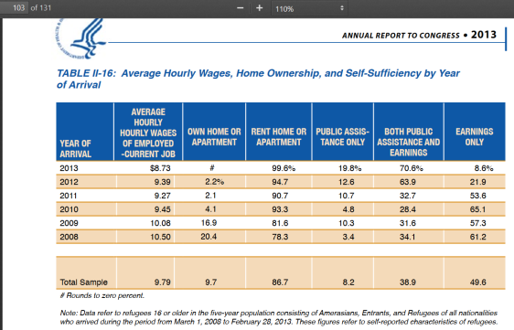
When judged by variables such as home ownership and the proportion of people who survive on public assistance, people who have stayed longer do better (Table II-16). But if you consider table II-17, a much larger proportion of the refugees surveyed in 2013 than in 2008 are partially dependent on public assistance, and it seems that a substantially smaller proportion of the refugees living in the US in the year 2013 was totally self-reliant than was the case 5 years earlier. Fortunately the 2013 report has a bit more data on this stuff (p. 107):

The table has more information on page 108, with more details about specific public assistance programs.Table II-22 includes data on how public assistance utilization has developed over time (it’s clear that utilization rates increased substantially during the half-decade observed):

Some related comments from the report:

“Use of non-cash assistance was generally higher than cash assistance. This is probably because Medicaid, the Supplemental Nutrition Assistance Program (SNAP), and housing assistance programs, though available to cash assistance households, also are available more broadly to households without children. SNAP utilization was lowest among Latin Americans (37 percent) but much higher for the other groups, reaching 89 to 91 percent among the refugees from Africa and the Middle East. […] Housing assistance varied by refugee group — as low as 4 percent for Latin American refugees and as high as 32 percent for refugees from South/Southeast Asia in the 2013 survey. In the same period, other refugee groups averaged use of housing assistance between 19 and 31 percent.” (pp. 107-108)

…

The report includes some specific data on Iraqi refugees – here’s one table from that section:

The employment rate of the Iraqis increased from 29.8% in the 2009 survey to 41.3% in 2013. However the US female employment rate is still actually not much different from the female employment rates you observe when you look at European data on these topics – just 29%, up from 18.8% in 2009. As a comparison, in the year 2010 the employment rate of Iraqi females living in Denmark was 28% (n=10163) (data from p.55 of the Statistics Denmark publication Indvandrere i Danmark 2011), almost exactly the same as the employment rate of female Iraqis in the US.

Of note in the context of the US data is perhaps also the fact that despite the employment rate going up for females in the time period observed, the labour market participation rate of this group actually decreased between 2009 and 2013, as it went from 42.2% to 38.1%. So more than 3 out of 5 Iraqi female refugees living in the US are outside the labour market, and almost one in four of those that are not are unemployed. A few observations from the report:

“The survey found that the overall EPR [employment rate, US] for the 2007 to 2009 Iraqi refugee group in the 2013 survey9 was 41 percent (55 percent for males and 29 percent for females), a steady increase in the overall rate from 39 percent in the 2012 survey, 36 percent in the 2011 survey, 31 percent in the 2010 survey, and 30 percent in the 2009 survey. As a point of further reference, the EPR for the general U.S. population was 58.5 percent in 2013, about 17 percentage points higher than that of the 2007 to 2009 Iraqi refugee group (41.3 percent). The U.S. male population EPR was nine percentage points higher than the rate for Iraqi males who arrived in the U.S. in 2007 to 2009 (64 percent versus 55 percent), while the rate for the Iraqi females who arrived in the U.S. in 2007 to 2009 was 24 points higher for all U.S. women (53 percent versus 29 percent). The difference between the male and female EPRs among the same group of Iraqi refugees (26 percentage points) also was much larger than the gap between male and female EPRs in the general U.S. population (11 points) […] The overall unemployment rate for the 2007 to 2009 Iraqi refugee group was 22.9 percent in the 2013 survey, about four times higher than that of the general U.S. population (6.5 percent) in 2013” (pp. 114-115).

Random Stuff

i. On the youtube channel of the Institute for Advanced Studies there has been a lot of activity over the last week or two (far more than 100 new lectures have been uploaded, and it seems new uploads are still being added at this point), and I’ve been watching a few of the recently uploaded astrophysics lectures. They’re quite technical, but you can watch them and follow enough of the content to have an enjoyable time despite not understanding everything:

This is a good lecture, very interesting. One major point made early on: “the take-away message is that the most common planet in the galaxy, at least at shorter periods, are planets for which there is no analogue in the solar system. The most common kind of planet in the galaxy is a planet with a radius of two Earth radii.” Another big take-away message is that small planets seem to be quite common (as noted in the conclusions, “16% of Sun-like stars have an Earth-sized planet”).

…

Of the lectures included in this post this was the one I liked the least; there are too many (‘obstructive’) questions/interactions between lecturer and attendants along the way, and the interactions/questions are difficult to hear/understand. If you consider watching both this lecture and the lecture below, I would say that it would probably be wise to watch the lecture below this one before you watch this one; I concluded that in retrospect some of the observations made early on in the lecture below would have been useful to know about before watching this lecture. (The first half of the lecture below was incidentally to me somewhat easier to follow than was the second half, but especially the first half hour of it is really quite good, despite the bad start (which one can always blame on Microsoft…)).

…

…

ii. Words I’ve encountered recently (…or ‘recently’ – it’s been a while since I last posted one of these lists): Divagations, periphrasis, reedy, architrave, sett, pedipalp, tout, togs, edentulous, moue, tatty, tearaway, prorogue, piscine, fillip, sop, panniers, auxology, roister, prepossessing, cantle, catamite, couth, ordure, biddy, recrudescence, parvenu, scupper, husting, hackle, expatiate, affray, tatterdemalion, eructation, coppice, dekko, scull, fulmination, pollarding, grotty, secateurs, bumf (I must admit that I like this word – it seems fitting, somehow, to use that word for this concept…), durophagy, randy, (brief note to self: Advise people having children who ask me about suggestions for how to name them against using this name (or variants such as Randi), it does not seem like a great idea), effete, apricity, sororal, bint, coition, abaft, eaves, gadabout, lugubriously, retroussé, landlubber, deliquescence, antimacassar, inanition.

…

iii. “The point of rigour is not to destroy all intuition; instead, it should be used to destroy bad intuition while clarifying and elevating good intuition. It is only with a combination of both rigorous formalism and good intuition that one can tackle complex mathematical problems; one needs the former to correctly deal with the fine details, and the latter to correctly deal with the big picture. Without one or the other, you will spend a lot of time blundering around in the dark (which can be instructive, but is highly inefficient). So once you are fully comfortable with rigorous mathematical thinking, you should revisit your intuitions on the subject and use your new thinking skills to test and refine these intuitions rather than discard them. One way to do this is to ask yourself dumb questions; another is to relearn your field.” (Terry Tao, There’s more to mathematics than rigour and proofs)

…

iv. A century of trends in adult human height. A figure from the paper (Figure 3 – Change in adult height between the 1896 and 1996 birth cohorts):

(Click to view full size. WordPress seems to have changed the way you add images to a blog post – if this one is even so annoyingly large, I apologize, I have tried to minimize it while still retaining detail, but the original file is huge). An observation from the paper:

“Men were taller than women in every country, on average by ~11 cm in the 1896 birth cohort and ~12 cm in the 1996 birth cohort […]. In the 1896 birth cohort, the male-female height gap in countries where average height was low was slightly larger than in taller nations. In other words, at the turn of the 20th century, men seem to have had a relative advantage over women in undernourished compared to better-nourished populations.”

I haven’t studied the paper in any detail but intend to do so at a later point in time.

…

v. I found this paper, on Exercise and Glucose Metabolism in Persons with Diabetes Mellitus, interesting in part because I’ve been very surprised a few times by offhand online statements made by diabetic athletes, who had observed that their blood glucose really didn’t drop all that fast during exercise. Rapid and annoyingly large drops in blood glucose during exercise have been a really consistent feature of my own life with diabetes during adulthood. It seems that there may be big inter-individual differences in terms of the effects of exercise on glucose in diabetics. From the paper:

“Typically, prolonged moderate-intensity aerobic exercise (i.e., 30–70% of one’s VO₂max) causes a reduction in glucose concentrations because of a failure in circulating insulin levels to decrease at the onset of exercise.¹² During this type of physical activity, glucose utilization may be as high as 1.5 g/min in adolescents with type 1 diabetes¹³ and exceed 2.0 g/min in adults with type 1 diabetes,¹⁴ an amount that quickly lowers circulating glucose levels. Persons with type 1 diabetes have large interindividual differences in blood glucose responses to exercise, although some intraindividual reproducibility exists.¹⁵ The wide ranging glycemic responses among individuals appears to be related to differences in pre-exercise blood glucose concentrations, the level of circulating counterregulatory hormones and the type/duration of the activity.²“

Civil Wars (II)

Here’s my first post about the book. In this post I’ll continue my coverage where I left off in my first post. A few of the chapters covered below I did not think very highly of, but other parts of the coverage are about as good as you could expect (given problems such as e.g. limited data etc.). Some of the stuff I found quite interesting. As people will note in the coverage below the book does address the religious dimension to some extent, though in my opinion far from to the extent that the variable deserves. An annoying aspect of the chapter on religion was to me that although the author of the chapter includes data which to me cannot but lead to some very obvious conclusions, the author seems to be very careful avoiding drawing those conclusions explicitly. It’s understandable, but still annoying. For related reasons I also got annoyed at him for presumably deliberately completely disregarding which seems in the context of his own coverage to be an actually very important component of Huntington’s thesis, that conflict at the micro level seems to very often be between muslims and ‘the rest’. Here’s a relevant quote from Clash…, p. 255:

“ethnic conflicts and fault line wars have not been evenly distributed among the world’s civilizations. Major fault line fighting has occurred between Serbs and Croats in the former Yugoslavia and between Buddhists and Hindus in Sri Lanka, while less violent conflicts took place between non-Muslim groups in a few other places. The overwhelming majority of fault line conflicts, however, have taken place along the boundary looping across Eurasia and Africa that separates Muslims from non-Muslims. While at the macro or global level of world politics the primary clash of civilizations is between the West and the rest, at the micro or local level it is between Islam and the others.”

This point, that conflict at the local level – which seems to be the type of conflict level you’re particularly interested in if you’re researching civil wars, as also argued in previous chapters in the coverage – according to Huntington seems to be very islam-centric, is completely overlooked (ignored?) in the handbook chapter, and if you haven’t read Huntington and your only exposure to him is through the chapter in question you’ll probably conclude that Huntington was wrong, because that seems to be the conclusion the author draws, arguing that other models are more convincing (I should add here that these other models do seem useful, at least in terms of providing (superficial) explanations; the point is just that I feel the author is misrepresenting Huntington and I dislike this). Although there are parts of the coverage in that chapter where I feel that it’s obvious the author and I do not agree, I should note that the fact that he talks about the data and the empirical research makes up for a lot of other stuff.

Anyway, on to the coverage – it’s perhaps worth noting, in light of the introductory remarks above, that the post has stuff on a lot of things besides religion, e.g. the role of natural resources, regime types, migration, and demographics.

…

“Elites seeking to end conflict must: (1) lead followers to endorse and support peaceful solutions; (2) contain spoilers and extremists and prevent them from derailing the process of peacemaking; and (3) forge coalitions with more moderate members of the rival ethnic group(s) […]. An important part of the two-level nature of the ethnic conflict is that each of the elites supporting the peace process be able to present themselves, and the resulting terms of the peace, as a “win” for their ethnic community. […] A strategy that a state may pursue to resolve ethnic conflict is to co-opt elites from the ethnic communities demanding change […]. By satisfying elites, it reduces the ability of the aggrieved ethnic community to mobilize. Such a process of co-option can also be used to strengthen ethnic moderates in order to undermine ethnic extremists. […] the co-opted elites need to be careful to be seen as still supporting ethnic demands or they may lose all credibility in their respective ethnic community. If this occurs, the likely outcome is that more extreme ethnic elites will be able to capture the ethnic community, possibly leading to greater violence.
It is important to note that “spoilers,” be they an individual or a small sub-group within an ethnic community, can potentially derail any peace process, even if the leaders and masses support peace (Stedman, 2001).”

“Three separate categories of international factors typically play into identity and ethnic conflict. The first is the presence of an ethnic community across state boundaries. Thus, a single community exists in more than one state and its demands become international. […] This division of an ethnic community can occur when a line is drawn geographically through a community […], when a line is drawn and a group moves into the new state […], or when a diaspora moves a large population from one state to another […] or when sub-groups of an ethnic community immigrate to the developed world […] When ethnic communities cross state boundaries, the potential for one state to support an ethnic community in the other state exists. […] There is also the potential for ethnic communities to send support to a conflict […] or to lobby their government to intervene […]. Ethnic groups may also form extra-state militias and cross international borders. Sometimes these rebel groups can be directly or indirectly sponsored by state governments, leading to a very complex situation […] A second set of possible international factors is non-ethnic international intervention. A powerful state may decide to intervene in an ethnic conflict for a variety of reasons, ranging from humanitarian support, to peacekeeping, to outright invasion […] The third and last factor is the commitment of non-governmental organizations (NGOs) or third-party mediators to a conflict. […] The record of international interventions in ethnic civil wars is quite mixed. There are many difficulties associated with international action [and] international groups cannot actually change the underlying root of the ethnic conflict (Lake and Rothchild, 1998; Kaufman, 1996).”

“A relatively simple way to think of conflict onset is to think that for a rebellion to occur two conditions need to be satisfactorily fulfilled: There must be a motivation and there must be an opportunity to rebel.3 First, the rebels need a motive. This can be negative – a grievance against the existing state of affairs – or positive – a desire to capture resource rents. Second, potential rebels need to be able to achieve their goal: The realization of their desires may be blocked by the lack of financial means. […] Work by Collier and Hoeffler (1998, 2004) was crucial in highlighting the economic motivation behind civil conflicts. […] Few conflicts, if any, can be characterized purely as “resource conflicts.” […] It is likely that few groups are solely motivated by resource looting, at least in the lower rank level. What is important is that valuable natural resources create opportunities for conflicts. To feed, clothe, and arm its members, a rebel group needs money. Unless the rebel leaders are able to raise sufficient funds, a conflict is unlikely to start no matter how severe the grievances […] As a consequence, feasibility of conflict – that is, valuable natural resources providing opportunity to engage in violent conflict – has emerged as a key to understanding the relation between valuable resources and conflict.”

“It is likely that some natural resources are more associated with conflict than others. Early studies on armed civil conflict used resource measures that aggregated different types of resources together. […] With regard to financing conflict start-up and warfare the most salient aspect is probably the ease with which a resource can be looted. Lootable resources can be extracted with simple methods by individuals or small groups, are easy to transport, and can be smuggled across borders with limited risks. Examples of this type of resources are alluvial gemstones and gold. By contrast, deep-shaft minerals, oil, and natural gas are less lootable and thus less likely sources of financing. […] Using comprehensive datasets on all armed civil conflicts in the world, natural resource production, and other relevant aspects such as political regime, economic performance, and ethnic composition, researchers have established that at least some high-value natural resources are related to higher risk of conflict onset. Especially salient in this respect seem to be oil and secondary diamonds[7] […] The results regarding timber […] and cultivation of narcotics […] are inconclusive. […] [An] important conclusion is that natural resources should be considered individually and not lumped together. Diamonds provide an illustrative example: the geological form of the diamond deposit is related to its effect on conflict. Secondary diamonds – the more lootable form of two deposit types – makes conflict more likely, longer, and more severe. Primary diamonds on the other hand are generally not related to conflict.”

“Analysis on conflict duration and severity confirm that location is a salient factor: resources matter for duration and severity only when located in the region where the conflict is taking place […] That the location of natural resources matters has a clear and important implication for empirical conflict research: relying on country-level aggregates can lead to wrong conclusions about the role of natural resources in armed civil conflict. As a consequence of this, there has been effort to collect location-specific data on oil, gas, drug cultivation, and gemstones”.

“a number of prominent studies of ethnic conflict have suggested that when ethnic groups grow at different rates, this may lead to fears of an altered political balance, which in turn might cause political instability and violent conflict […]. There is ample anecdotal evidence for such a relationship [but unfortunately little quantitative research…]. The civil war in Lebanon, for example, has largely been attributed to a shift in the delicate ethnic balance in that state […]. Further, in the early 1990s, radical Serb leaders were agitating for the secession of “Serbian” areas in Bosnia-Herzegovina by instigating popular fears that Serbs would soon be outnumbered by a growing Muslim population heading for the establishment of a Shari’a state”.

“[One] part of the demography-conflict literature has explored the role of population movements. Most of this literature […] treats migration and refugee flows as a consequence of conflict rather than a potential cause. Some scholars, however, have noted that migration, and refugee migration in particular, can spur the spread of conflict both between and within states […]. Existing work suggests that environmentally induced migration can lead to conflict in receiving areas due to competition for scarce resources and economic opportunities, ethnic tensions when migrants are from different ethnic groups, and exacerbation of socioeconomic “fault lines” […] Salehyan and Gleditsch (2006) point to spill-over effects, in the sense that mass refugee migration might spur tensions in neighboring or receiving states by imposing an economic burden and causing political stability [sic]. […] Based on a statistical analysis of refugees from neighboring countries and civil war onset during the period 1951–2001, they find that countries that experience an influx of refugees from neighboring states are significantly more likely to experience wars themselves. […] While the youth bulge hypothesis [large groups of young males => higher risk of violence/war/etc.] in general is supported by empirical evidence, indicating that countries and areas with large youth cohorts are generally at a greater risk of low-intensity conflict, the causal pathways relating youth bulges to increased conflict propensity remain largely unexplored quantitatively. When it comes to the demographic factors which have so far received less attention in terms of systematic testing – skewed sex ratios, differential ethnic growth, migration, and urbanization – the evidence is somewhat mixed […] a clear challenge with regard to the study of demography and conflict pertains to data availability and reliability. […] Countries that are undergoing armed conflict are precisely those for which we need data, but also those in which census-taking is hampered by violence.”

“Most research on the duration of civil war find that civil wars in democracies tend to be longer than other civil wars […] Research on conflict severity finds some evidence that democracies tend to see fewer battledeaths and are less likely to target civilians, suggesting that democratic institutions may induce some important forms of restraints in armed conflict […] Many researchers have found that democratization often precedes an increase in the risk of the onset of armed conflict. Hegre et al. (2001), for example, find that the risk of civil war onset is almost twice as high a year after a regime change as before, controlling for the initial level of democracy […] Many argue that democratic reforms come about when actors are unable to rule unilaterally and are forced to make concessions to an opposition […] The actual reforms to the political system we observe as democratization often do not suffice to reestablish an equilibrium between actors and the institutions that regulate their interactions; and in its absence, a violent power struggle can follow. Initial democratic reforms are often only partial, and may fail to satisfy the full demands of civil society and not suffice to reduce the relevant actors’ motivation to resort to violence […] However, there is clear evidence that the sequence matters and that the effect [the increased risk of civil war after democratization, US] is limited to the first election. […] civil wars […] tend to be settled more easily in states with prior experience of democracy […] By our count, […] 75 percent of all annual observations of countries with minor or major armed conflicts occur in non-democracies […] Democracies have an incidence of major armed conflict of only 1 percent, whereas nondemocracies have a frequency of 5.6 percent.”

“Since the Iranian revolution in the late 1970s, religious conflicts and the rise of international terror organizations have made it difficult to ignore the facts that religious factors can contribute to conflict and that religious actors can cause or participate in domestic conflicts. Despite this, comprehensive studies of religion and domestic conflict remain relatively rare. While the reasons for this rarity are complex there are two that stand out. First, for much of the twentieth century the dominant theory in the field was secularization theory, which predicted that religion would become irrelevant and perhaps extinct in modern times. While not everyone agreed with this extreme viewpoint, there was a consensus that religious influences on politics and conflict were a waning concern. […] This theory was dominant in sociology for much of the twentieth century and effectively dominated political science, under the title of modernization theory, for the same period. […] Today supporters of secularization theory are clearly in the minority. However, one of their legacies has been that research on religion and conflict is a relatively new field. […] Second, as recently as 2006, Brian Grim and Roger Finke lamented that “religion receives little attention in international quantitative studies. Including religion in cross-national studies requires data, and high-quality data are in short supply” […] availability of the necessary data to engage in quantitative research on religion and civil wars is a relatively recent development.”

“[Some] studies [have] found that conflicts involving actors making religious demands – such as demanding a religious state or a significant increase in religious legislation – were less likely to be resolved with negotiated settlements; a negotiated settlement is possible if the settlement focused on the non-religious aspects of the conflict […] One study of terrorism found that terror groups which espouse religious ideologies tend to be more violent (Henne, 2012). […] The clear majority of quantitative studies of religious conflict focus solely on inter-religious conflicts. Most of them find religious identity to influence the extent of conflict […] but there are some studies which dissent from this finding”.

“Terror is most often selected by groups that (1) have failed to achieve their goals through peaceful means, (2) are willing to use violence to achieve their goals, and (3) do not have the means for higher levels of violence.”

“the PITF dataset provides an accounting of the number of domestic conflicts that occurred in any given year between 1960 and 2009. […] Between 1960 and 2009 the modified dataset includes 817 years of ethnic war, 266 years of genocides/politicides, and 477 years of revolutionary wars. […] Cases were identified as religious or not religious based on the following categorization:
1 Not Religious.
2 Religious Identity Conflict: The two groups involved in the conflict belong to different religions or different denominations of the same religion.[11]
3 Religious Wars: The two sides of the conflict belong to the same religion but the description of the conflict provided by the PITF project identifies religion as being an issue in the conflict. This typically includes challenges by religious fundamentalists to more secular states. […]
The results show that both numerically and as a proportion of all conflict, religious state failures (which include both religious identity conflicts and religious wars) began increasing in the mid-1970s. […] As a proportion of all conflict, religious state failures continued to increase and became a majority of all state failures in 2002. From 2002 onward, religious state failures were between 55 percent and 62 percent of all state failures in any given year.”

“Between 2002 and 2009, eight of 12 new state failures were religious. All but one of the new religious state failures were ongoing as of 2009. These include:
• 2002: A rebellion in the Muslim north of the Ivory Coast (ended in 2007)
• 2003: The beginning of the Sunni–Shia violent conflict in Iraq (ongoing)
• 2003: The resumption of the ethnic war in the Sudan [97% muslims, US] (ongoing)
• 2004: Muslim militants challenged Pakistan’s government in South and North Waziristan. This has been followed by many similar attacks (ongoing)
• 2004: Outbreak of violence by Muslims in southern Thailand (ongoing)
• 2004: In Yemen [99% muslims, US], followers of dissident cleric Husain Badr al-Din al-Huthi create a stronghold in Saada. Al-Huthi was killed in September 2004, but serious fighting begins again in early 2005 (ongoing)
• 2007: Ethiopia’s invasion of southern Somalia causes a backlash in the Muslim (ethnic- Somali) Ogaden region (ongoing)
• 2008: Islamist militants in the eastern Trans-Caucasus region of Russia bordering on Georgia (Chechnya, Dagestan, and Ingushetia) reignited their violent conflict against Russia[12] (ongoing)” [my bold]

“There are few additional studies which engage in this type of longitudinal analysis. Perhaps the most comprehensive of such studies is presented in Toft et al.’s (2011) book God’s Century based on data collected by Toft. They found that religious conflicts – defined as conflicts with a religious content – rose from 19 percent of all civil wars in the 1940s to about half of civil wars during the first decade of the twenty-first century. Of these religious conflicts, 82 percent involved Muslims. This analysis includes only 135 civil wars during this period. The lower number is due to a more restrictive definition of civil war which includes at least 1,000 battle deaths. This demonstrates that the findings presented above also hold when looking at the most violent of civil wars.” [my bold]

Stuff/Links/Open Thread

i. National Health Statistics Reports, Number 49, March 22, 2012 – First Marriages in the United States: Data From the 2006–2010 National Survey of Family Growth.

“This report shows trends and group differences in current marital status, with a focus on first marriages among women and men aged 15–44 years in the United States. Trends and group differences in the timing and duration of first marriages are also discussed. […] The analyses presented in this report are based on a nationally representative sample of 12,279 women and 10,403 men aged 15–44 years in the household population of the United States.”

“In 2006–2010, […] median age at first marriage was 25.8 for women and 28.3 for men.”

“Among women, 68% of unions formed in 1997–2001 began as a cohabitation rather than as a marriage (8). If entry into any type of union, marriage or cohabitation, is taken into account, then the timing of a first union occurs at roughly the same point in the life course as marriage did in the past (9). Given the place of cohabitation in contemporary union formation, descriptions of marital behavior, particularly those concerning trends over time, are more complete when cohabitation is also measured. […] Trends in the current marital statuses of women using the 1982, 1995, 2002, and 2006–2010 NSFG indicate that the percentage of women who were currently in a first marriage decreased over the past several decades, from 44% in 1982 to 36% in 2006–2010 […]. At the same time, the percentage of women who were currently cohabiting increased steadily from 3.0% in 1982 to 11% in 2006– 2010. In addition, the proportion of women aged 15–44 who were never married at the time of interview increased from 34% in 1982 to 38% in 2006–2010.”

“In 2006–2010, the probability of first marriage by age 25 was 44% for women compared with 59% in 1995, a decrease of 25%. By age 35, the probability of first marriage was 84% in 1995 compared with 78% in 2006–2010 […] By age 40, the difference in the probability of age at first marriage for women was not significant between 1995 (86%) and 2006–2010 (84%). These findings suggest that between 1995 and 2006– 2010, women married for the first time at older ages; however, this delay was not apparent by age 40.”

“In 2006–2010, the probability of a first marriage lasting at least 10 years was 68% for women and 70% for men. Looking at 20 years, the probability that the first marriages of women and men will survive was 52% for women and 56% for men in 2006–2010. These levels are virtually identical to estimates based on vital statistics from the early 1970s (24). For women, there was no significant change in the probability of a first marriage lasting 20 years between the 1995 NSFG (50%) and the 2006–2010 NSFG (52%)”

“Women who had no births when they married for the first time had a higher probability of their marriage surviving 20 years (56%) compared with women who had one or more births at the time of first marriage (33%). […] Looking at spousal characteristics, women whose first husbands had been previously married (38%) had a lower probability of their first marriage lasting 20 years compared with women whose first husband had never been married before (54%). Women whose first husband had children from previous relationships had a lower probability that their first marriage would last 20 years (37%) compared with first husbands who had no other children (54%). For men, […] patterns of first marriage survival […] are similar to those shown for women for marriages that survived up to 15 years.”

“These data show trends that are consistent with broad demographic changes in the American family that have occurred in the United States over the last several decades. One such trend is an increase in the time spent unmarried among women and men. For women, there was a continued decrease in the percentage currently married for the first time — and an increase in the percent currently cohabiting — in 2006–2010 compared with earlier years. For men, there was also an increase in the percentage unmarried and in the percentage currently cohabiting between 2002 and 2006–2010. Another trend is an increase in the age at first marriage for women and men, with men continuing to marry for the first time at older ages than women. […] Previous research suggests that women with more education and better economic prospects are more likely to delay first marriage to older ages, but are ultimately more likely to become married and to stay married […]. Data from the 2006–2010 NSFG support these findings”

…

ii. Involuntary Celibacy: A life course analysis (review). This is not a link to the actual paper – the paper is not freely available, which is why I do not link to it – but rather a link to a report talking about what’s in that paper. However I found some of the stuff interesting:

“A member of an on-line discussion group for involuntary celibates approached the first author of the paper via email to ask about research on involuntary celibacy. It soon became apparent that little had been done, and so the discussion group volunteered to be interviewed and a research team was put together. An initial questionnaire was mailed to 35 group members, and they got a return rate of 85%. They later posted it to a web page so that other potential respondents had access to it. Eventually 60 men and 22 women took the survey.”

“Most were between the ages of 25-34, 28% were married or living with a partner, 89% had attended or completed college. Professionals (45%) and students (16%) were the two largest groups. 85% of the sample was white, 89% were heterosexual. 70% lived in the U.S. and the rest primarily in Western Europe, Canada and Australia. […] the value of this research lies in the rich descriptive data obtained about the lives of involuntary celibates, a group about which little is known. […] The questionnaire contained 13 categorical, close-ended questions assessing demographic data such as age, sex, marital status, living arrangement, income, education, employment type, area of residence, race/ethnicity, sexual orientation, religious preference, political views, and time spent on the computer. 58 open-ended questions investigated such areas as past sexual experiences, current relationships, initiating relationships, sexuality and celibacy, nonsexual relationships and the consequences of celibacy. They started out by asking about childhood experiences, progressed to questions about teen and early adult years and finished with questions about current status and the effects of celibacy.”

“78% of this sample had discussed sex with friends, 84% had masturbated as teens. The virgins and singles, however, differed from national averages in their dating and sexual experiences.”

“91% of virgins and 52 % of singles had never dated as teenagers. Males reported hesitancy in initiating dates, and females reporting a lack of invitations by males. For those who did date, their experiences tended to be very limited. Only 29% of virgins reported first sexual experiences that involved other people, and they frequently reported no sexual activity at all except for masturbation. Singles were more likely than virgins to have had an initial sexual experience that involved other people (76%), but they tended to report that they were dissatisfied with the experience. […] While most of the sample had discussed sex with friends and masturbated as teens, most virgins and singles did not date. […] Virgins and singles may have missed important transitions, and as they got older, their trajectories began to differ from those of their age peers. Patterns of sexuality in young adulthood are significantly related to dating, steady dating and sexual experience in adolescence. It is rare for a teenager to initiate sexual activity outside of a dating relationship. While virginity and lack of experience are fairly common in teenagers and young adults, by the time these respondents reached their mid-twenties, they reported feeling left behind by age peers. […] Even for the heterosexuals in the study, it appears that lack of dating and sexual experimentation in the teen years may be precursors to problems in adult sexual relationships.”

“Many of the virgins reported that becoming celibate involved a lack of sexual and interpersonal experience at several different transition points in adolescence and young adulthood. They never or rarely dated, had little experience with interpersonal sexual activity, and had never had sexual intercourse. […] In contrast, partnered celibates generally became sexually inactive by a very different process. All had initially been sexually active with their partners, but at some point stopped. At the time of the survey, sexual intimacy no longer or very rarely occurred in their relationships. The majority of them (70%) started out having satisfactory relationships, but they slowly stopped having sex as time went on.”

“shyness was a barrier to developing and maintaining relationships for many of the respondents. Virgins (94%) and singles (84%) were more likely to report shyness than were partnered respondents (20%). The men (89%) were more likely to report being shy than women (77%). 41% of virgins and 23% of singles reported an inability to relate to others socially. […] 1/3 of the respondents thought their weight, appearance, or physical characteristics were obstacles to attracting potential partners. 47% of virgins and 56% of singles mentioned these factors, compared to only 9% of partnered people. […] Many felt that their sexual development had somehow stalled in an earlier stage of life; feeling different from their peers and feeling like they will never catch up. […] All respondents perceived their lack of sexual activity in a negative light and in all likelihood, the relationship between involuntary celibacy and unhappiness, anger and depression is reciprocal, with involuntary celibacy contributing to negative feelings, but these negative feelings also causing people to feel less self-confident and less open to sexual opportunities when they occur. The longer the duration of the celibacy, the more likely our respondents were to view it as a permanent way of life. Virginal celibates tended to see their condition as temporary for the most part, but the older they were, the more likely they were to see it as permanent, and the same was true for single celibates.”

It seems to me from ‘a brief look around’ that not a lot of research has been done on this topic, which I find annoying. Because yes, I’m well aware these are old data and that the sample is small and ‘convenient’. Here’s a brief related study on the ‘Characteristics of adult women who abstain from sexual intercourse‘ – the main findings:

“Of the 1801 respondents, 244 (14%) reported abstaining from intercourse in the past 6 months. Univariate analysis revealed that abstinent women were less likely than sexually active women to have used illicit drugs [odds ratio (OR) 0.47; 95% CI 0.35–0.63], to have been physically abused (OR 0.44, 95% CI 0.31–0.64), to be current smokers (OR 0.59, 95% CI 0.45–0.78), to drink above risk thresholds (OR 0.66, 95% CI 0.49–0.90), to have high Mental Health Inventory-5 scores (OR 0.7, 95% CI 0.54–0.92) and to have health insurance (OR 0.74, 95% CI 0.56–0.98). Abstinent women were more likely to be aged over 30 years (OR 1.98, 95% CI 1.51–2.61) and to have a high school education (OR 1.38, 95% CI 1.01–1.89). Logistic regression showed that age >30 years, absence of illicit drug use, absence of physical abuse and lack of health insurance were independently associated with sexual abstinence.

Conclusions

Prolonged sexual abstinence was not uncommon among adult women. Periodic, voluntary sexual abstinence was associated with positive health behaviours, implying that abstinence was not a random event. Future studies should address whether abstinence has a causal role in promoting healthy behaviours or whether women with a healthy lifestyle are more likely to choose abstinence.”

Here’s another more recent study – Prevalence and Predictors of Sexual Inexperience in Adulthood (unfortunately I haven’t been able to locate a non-gated link) – which I found and may have a closer look at later. A few quotes/observations:

“By adulthood, sexual activity is nearly universal: 97 % of men and 98 % of women between the ages of 25-44 report having had vaginal intercourse (Mosher, Chandra, & Jones, 2005). […] Although the majority of individuals experience this transition during adolescence or early adulthood, a small minority remain sexually inexperienced far longer. Data from the NSFG indicate that about 5% of males and 3% of females between the ages of 25 and 29 report never having had vaginal sex (Mosher et al., 2005). While the percentage of sexually inexperienced participants drops slightly among older age groups, between 1 and 2% of both males and females continue to report that they have never had vaginal sex even into their early 40s. Other nationally representative surveys have yielded similar estimates of adult sexual inexperience (Billy, Tanfer, Grady, & Klepinger, 1993)”

“Individuals who have not experienced any type of sexual activity as adults […] may differ from those who only abstain from vaginal intercourse. For example, vaginal virgins who engage in “everything but” vaginal sex – sometimes referred to as “technical virgins” […] – may abstain from vaginal sex in order to avoid its potential negative consequences […]. In contrast, individuals who have neither coital nor noncoital experience may have been unable to attract sexual partners or may have little interest in sexual involvement. Because prior analyses have generally conflated these two populations, we know virtually nothing about the prevalence or characteristics of young adults who have abstained from all types of sexual activity.”

“We used data from 2,857 individuals who participated in Waves I–IV of the National Longitudinal Study of Adolescent Health (Add Health) and reported no sexual activity (i.e., oral-genital, vaginal, or anal sex) by age 18 to identify, using discrete-time survival models, adolescent sociodemographic, biosocial, and behavioral characteristics that predicted adult sexual inexperience. The mean age of participants at Wave IV was 28.5 years (SD = 1.92). Over one out of eight participants who did not initiate sexual activity during adolescence remained abstinent as young adults. Sexual non-attraction significantly predicted sexual inexperience among both males (aOR = 0.5) and females (aOR = 0.6). Males also had lower odds of initiating sexual activity after age 18 if they were non-Hispanic Asian, reported later than average pubertal development, or were rated as physically unattractive (aORs = 0.6–0.7). Females who were overweight, had lower cognitive performance, or reported frequent religious attendance had lower odds of sexual experience (aORs = 0.7–0.8) while those who were rated by the interviewers as very attractive or whose parents had lower educational attainment had higher odds of sexual experience (aORs = 1.4–1.8). Our findings underscore the heterogeneity of this unique population and suggest that there are a number of different pathways that may lead to either voluntary or involuntary adult sexual inexperience.”

…

iii. Association between breastfeeding and intelligence, educational attainment, and income at 30 years of age: a prospective birth cohort study from Brazil.

“Breastfeeding has clear short-term benefits, but its long-term consequences on human capital are yet to be established. We aimed to assess whether breastfeeding duration was associated with intelligence quotient (IQ), years of schooling, and income at the age of 30 years, in a setting where no strong social patterning of breastfeeding exists. […] A prospective, population-based birth cohort study of neonates was launched in 1982 in Pelotas, Brazil. Information about breastfeeding was recorded in early childhood. At 30 years of age, we studied the IQ (Wechsler Adult Intelligence Scale, 3rd version), educational attainment, and income of the participants. For the analyses, we used multiple linear regression with adjustment for ten confounding variables and the G-formula. […] From June 4, 2012, to Feb 28, 2013, of the 5914 neonates enrolled, information about IQ and breastfeeding duration was available for 3493 participants. In the crude and adjusted analyses, the durations of total breastfeeding and predominant breastfeeding (breastfeeding as the main form of nutrition with some other foods) were positively associated with IQ, educational attainment, and income. We identified dose-response associations with breastfeeding duration for IQ and educational attainment. In the confounder-adjusted analysis, participants who were breastfed for 12 months or more had higher IQ scores (difference of 3,76 points, 95% CI 2,20–5,33), more years of education (0,91 years, 0,42–1,40), and higher monthly incomes (341,0 Brazilian reals, 93,8–588,3) than did those who were breastfed for less than 1 month. The results of our mediation analysis suggested that IQ was responsible for 72% of the effect on income.”

This is a huge effect size.

…

iv. Grandmaster blunders (chess). This is quite a nice little collection; some of the best players in the world have actually played some really terrible moves over the years, which I find oddly comforting in a way..

…

v. History of the United Kingdom during World War I (wikipedia, ‘good article’). A few observations from the article:

“In 1915, the Ministry of Munitions under David Lloyd-George was formed to control munitions production and had considerable success.^[113][114] By April 1915, just two million rounds of shells had been sent to France; by the end of the war the figure had reached 187 million,^[115] and a year’s worth of pre-war production of light munitions could be completed in just four days by 1918.”

“During the war, average calories intake [in Britain] decreased only three percent, but protein intake six percent.^[47]“

“Energy was a critical factor for the British war effort. Most of the energy supplies came from coal mines in Britain, where the issue was labour supply. Critical however was the flow of oil for ships, lorries and industrial use. There were no oil wells in Britain so everything was imported. The U.S. pumped two-thirds of the world’s oil. In 1917, total British consumption was 827 million barrels, of which 85 percent was supplied by the United States, and 6 percent by Mexico.”

“In the post war publication Statistics of the Military Effort of the British Empire During the Great War 1914–1920 (The War Office, March 1922), the official report lists 908,371 ‘soldiers’ as being either killed in action, dying of wounds, dying as prisoners of war or missing in action in the World War. (This is broken down into the United Kingdom and its colonies 704,121; British India 64,449; Canada 56,639; Australia 59,330; New Zealand 16,711; South Africa 7,121.) […] The civilian death rate exceeded the prewar level by 292,000, which included 109,000 deaths due to food shortages and 183,577 from Spanish Flu.”

…

vi. House of Plantagenet (wikipedia, ‘good article’).

…

vii. r/Earthp*rn. There are some really nice pictures here…

Personal Relationships (4)

Here’s a previous post about the book, with links to other posts in the series.

I decided in this post to have a look at a few of the chapters in the first part(s) of the book. As earlier mentioned I lost my notes and highlights to these parts of the book due to computer trouble, making it much more difficult and time consuming to blog this stuff, but I wanted to cover some of that stuff even so because if I don’t I’ll forget the details (to the extent that I have not already – I should caution that this post provides relatively ‘lazy coverage’ as I felt it to be completely out of the question to select material from the book to talk about here using the same criteria I normally employ).

…

An obvious but important conclusion from the chapter on The Affective Structure of Marriage, which is a chapter that among other things covers multiple conceptual models dealing with relationship change, is that: “various models of marital change are useful because no single pathway describes changes in all, or even most, marriages. Even among couples sharing a similar outcome (e.g., divorce), there is considerable variation in the course toward that outcome. This implies that attempts to develop a single explanation or description of divorce are likely to be, at best, incomplete. Concluding that multiple models are useful is merely recognizing that there are multiple developmental processes in marriage.” Relationships may change for all sorts of reasons, and there is no full model out there which explains everything. This stuff is complicated. It’s noted in the chapter that some of the attempts people have made at trying to e.g. predict which couples divorced over a given time period turned out to perform really quite well on one sample (using longitudinal data – this is not just unsophisticated cross section analyses we’re dealing with), but then it turned out later that they perform really quite horribly on validation samples using the same type of data to predict outcomes in different couples. Similar stimuli may have different effects depending on how long people have been together. Different models deal with time frame aspects in different ways.

I’ll mention a few results from the literature covered in that chapter here. One is that couples who were initially more affectionate and less antagonistic were happier 13 years later than were other couples who were still together at that point in time but had lower initial levels of affection/higher antagonism. It’s also been found that couples which are high in antagonism early on in the relationship (‘lots of drama’) are more likely to divorce early on; disillusionment after a few years of marriage seems to be a better predictor of divorce years later, with initial affection being an important moderating variable in the sense that couples who were initially higher in affection were together for a longer period of time before they eventually divorced. Shorter relationship duration at the time of marriage seems to predict divorce. Personality characteristics such as (trait) (presumably also state-, US) anxiety and neuroticism are associated with relationship dissatisfaction and divorce risk. I should probably once again emphasize that the only reason why I’m not providing effect sizes here is that the authors do not, and so I’m not able to. Some conclusions from the chapter:

“one of the most exciting nascent trends in the marital literature involves the recognition that there is not a single unitary process leading to marital distress and divorce […]. Some couples begin marriage with lower marital satisfaction than most other couples but remain married indefinitely, whereas other couples begin marriage very satisfied but end up divorcing. Moreover, the predictors of dissatisfaction and divorce are not always the same; for instance, stable characteristics such as trait anxiety appear to be more strongly related to satisfaction than they are to divorce […]. Even the processes leading to divorce are not uniform, with some couples who eventually divorce beginning marriage with high levels of hostility and divorcing quickly, others beginning marriage with moderate amounts of both positive and negative elements before becoming quite low in affection, and still others beginning marriage with exceedingly high levels of affection that are not sustained over the early years of marriage. Also, the predictors of divorce are different for divorces that occur earlier in marriage compared with those that happen later in marriage. […] Being high in conscientiousness [for example] appears to diminish the chances that one will divorce early in marriage but does not appear to prevent eventual divorce”.

It should be noted, as they also do, that much of this research is based on what they in the book call ‘observational data’, which in this context means data obtained by actually observing the individuals, usually in a lab, and then coding specific behaviours in specific ways. They didn’t just ask people if they were affectionate towards each other; they tried to estimate whether or not they were, based on behaviours they could observe. There are problems with this sort of data and they talk about that in the chapter; for example it has been argued (I think I may have talked about this before in my coverage) that the most effective kind of support may well be invisible support (“actions that take place outside the recipients’ awareness”, or supportive actions which are provided “in such a skillful way that, although the information about the transaction is available to the recipient, the transaction is not coded as enacted support”) – and this sort of support is difficult to observe in a lab; whereas on the other hand the most visible sort of support, which is the easiest type to code by observers, may be counterproductive (such actions may provide a signal to the partner that the other party considers him/her too incompetent to handle the task on his/her own, which may lead to self-doubt etc. in the recipient), perhaps making interpretations slightly more difficult than one might think they are. A related problem seems to me to be that not providing support may in some situations be the optimal approach to take by the partner (‘my partner obviously doesn’t need my help right now, and if I were to provide support in this situation this would not be helpful’), and so such behaviours may be indicative of a strong relationship – yet that’s not how such behaviours will be coded in the studies. There are some problems here.

Next, a few observations dealing with divorce and postdivorce relationships. This data is old, but better than nothing: “Most divorced adults find another romantic partner. In the United States, the probability of cohabiting after the dissolution of first marriage is 70% after 10 years […] Census estimates project that in the United States nearly 85% of divorced people remarry […]. Although the remarriage rate is lower in other Western societies, most divorced people eventually cohabit or remarry […] It is an almost universal finding that children have more difficulty adapting to parental remarriage than do the adults.” I thought I should mention in a slightly unrelated context that I recently came across a Danish article about how children are dealt with here in the divorce context; I was not surprised to learn that women get custody in 90% of the cases – the politicians are thinking about changing this (this did surprise me), which has caused some organizations to argue that it’s a bad idea to change this state of affairs (again, not surprising). I’ve blogged US data on this stuff before – go have a look at the archives/use the search function if you’re curious, I’m too lazy to provide a link. I believe the US numbers are reasonably similar. An important observation made in the chapter is that parenting roles have evolved over time, and that the institutional setup had not really evolved with them at the time this book was written: “Child support policies have been predicated on the notion of fathers having only one set of children to support. In fact, increases in multiple marital and cohabiting relationships means that nearly 75% of remarried men have multiple sets of children to support (emotionally and financially) both inside and outside their current relationship.” It’s important to observe in this context that the proportion of all marriages which were remarriages was really high in the US, and that the remarried couples made up a big proportion of the total: “About half of all U.S. marriages are remarriages for one or both partners” (data from the U.S. Census Bureau, 2000). Things may or may not be different today.

Some observations from the chapter about personal relationships in adolescence and early adulthood: “Friendships and romantic relationships are tightly interwoven in adolescence and early adulthood. Unsupervised mixed-gender peer groups during adolescence provide opportunities and supportive environments for “pairing off” between group members. By mid-adolescence, most individuals have been involved in at least one romantic relationship; by the early years of early adulthood, most are currently participating in an ongoing romantic relationship (Collins, 2003). […] Existing findings point to a shift in the qualitative characteristics of dating relationships between the ages of 15 and 17 years, and dating among early adults seems similar in key ways to dating among late adolescents. After age 17, the likelihood of being involved in a romantic relationship changes little […] Having a romantic relationship and the quality of that relationship are associated positively with romantic self-concept and, in turn, with feelings of self-worth […], and longitudinal evidence indicates that by late adolescence, self-perceived competence in romantic relationships emerges as a reliable component of general competence […]. Whether adolescent romantic relationships play a distinctive role in identity formation during adolescence is not known, although considerable speculation and some theoretical contentions imply a link […] The most widely studied patterns have to do with variations in the timing of involvement in both romantic relationships and sexual activity, typically showing that early dating and sexual activity are risk factors for current and later problem behaviors and social and emotional difficulties […] The social worlds of those involved in romantic relationships differ from those who are not because romantic partners quickly become dominant in the relationship hierarchy […]. Although romantic interconnections initially are predicated on principles of social exchange, commitment drives participants to transform this voluntary relationship into one that is more obligatory and permanent […]. Eventually, most early adults marry and reproduce, further transforming the relationship and marginalizing remaining friendships, thus effectively ending the peer group’s dominance of relationship experiences”.

And finally some data and observations from the chapter about close relationships in middle and late adulthood: “The majority of adults in the United States are married, but the proportion is smaller in old age than earlier in adulthood (ages 35 to 54 years = 71.3%, 55 to 64 years = 74.2%, and 65 or older = 56.7%), and a notable sex difference in the proportion married exists between men and women aged 65 or older (75.7% versus 42.9%, respectively). The majority of households comprise family households (68%), usually of married couples (52%), but 32% of adults live in non-family households, including the 26% who live alone [do keep in mind that many of those 26% are involved in romantic relationships as well, though the characteristics of the relationships they have are different]. Among persons aged 75 years or older, however, the proportion living alone is much higher (39.6%) because of the greater likelihood of being widowed (ages 35 to 54 years = 1.6%, 55 to 64 years = 6.7%, 65 to 74 = 19.6%, and 75 or older = 41%, U.S. Census Bureau, 2003). […] the proportion of householders with children of any age at home remains above 50% even in the 45- to 54-year-old age group (Russell, 2001). […] One of the key findings of research on the causes and consequences of relational difficulties in adulthood is that negative dimensions of interactions have stronger effects than positive ones on relationship quality and satisfaction.”

Sexually Transmitted Diseases (4th edition) (III)

I read the first nine chapters of this very long book a while back, and I decided to have another go at it. I have now read chapters 10-18, the first seven of which deal with ‘Profiles of Vulnerable Populations’ (including chapters about: Gender and Sexually Transmitted Diseases (10), Adolescents and STDs Including HIV Infection (11), Female Sex Workers and Their Clients in the Epidemiology and Control of Sexually Transmitted Diseases (12), Homosexual and Bisexual Behavior in Men in Relation to STDs and HIV Infection (13), Lesbian Sexual Behavior in Relation to STDs and HIV Infection (14) (some surprising stuff in that chapter, but I won’t cover that here), HIV and Other Sexually Transmitted Infections in Injection Drug Users and Crack Cocaine Smokers (15), and STDs, HIV/AIDS, and Migrant Populations (16)), and the last two of which deal with ‘Host Immunity and Molecular Pathogenesis and STD’ (Chapters about: ‘Genitourinary Immune Defense’ (17) and ‘Normal Genital Flora’ (19 as well as ‘Pathogenesis of Sexually Transmitted Viral and Bacterial Infections’ (19) – I have only read the first two chapters in that section so far, and so I won’t cover the last chapter here. I also won’t cover the content of the first of these chapters, but for different reasons). The book has 108 chapters and more than 2000 pages, so although I’ve started reading the book again I’m sure I won’t finish the book this time either. My interest in the things covered in this book is purely academical in the first place.

You can read my first two posts about the book here and here.

Some observations and comments below…

…

“A major problem when assessing the risk of men and women of contracting an STI [sexually transmitted infection], is the differential reporting of sexual behavior between men and women. It is believed that women tend to underreport sexual activity, whereas men tend to over-report. This has been highlighted by studies assessing changes in reported age at first sexual intercourse between successive birth cohorts¹⁵ and by studies that compared the numbers of sex partners reported by men and by women.¹⁰,¹³,¹⁶, ¹⁷, ¹⁸ […] There is widespread agreement that women are more frequently and severely affected by STIs than men. […] In the studies in the general population that have assessed the prevalence of gonorrhea, chlamydial infection, and active syphilis, the prevalence was generally higher in women than in men […], with differences in prevalence being more marked in the younger age groups. […] HIV infection is also strikingly more prevalent in women than in men in most populations where the predominant mode of transmission is heterosexual intercourse and where the HIV epidemic is mature […] It is generally accepted that the male-to-female transmission of STI pathogens is more efficient than female-to-male transmission. […] The high vulnerability to STIs of young women compared to young men is [however] the result of an interplay between psychological, sociocultural, and biological factors.³³”

“Complications of curable STIs, i.e., STIs caused by bacteria or protozoa, can be avoided if infected persons promptly seek care and are managed appropriately. However, a prerequisite to seeking care is that infected persons are aware that they are infected and that they seek treatment. A high proportion of men and of women infected with N. gonorrhoeae, C. trachomatis, or T. vaginalis, however, never experience symptoms. Women are asymptomatic more often than men. It has been estimated that 55% of episodes of gonorrhea in men and 86% of episodes in women remain asymptomatic; 89% of men with chlamydial infection remain asymptomatic and 94% of women.⁶⁶ For chlamydial infection, it has been well documented that serious complications, including infertility due to tubal occlusion, can occur in the absence of a history of symptoms of pelvic inflammatory disease.⁶⁵”

“Most population-based STD rates underestimate risk for sexually active adolescents because the rate is inappropriately expressed as cases of disease divided by the number of individuals in this age group. Yet only those who have had intercourse are truly at risk for STDs. For rates to reflect risk among those who are sexually experienced, appropriate denominators should include only the number of individuals in the demographic group who have had sexual intercourse. […] In general, when rates are corrected for those who are sexually active, the youngest adolescents have the highest STD rates of any age group.⁵”

“Although risk of HPV acquisition increases with number of partners,⁶⁷,⁷⁴,⁷⁵ prevalence of infection is substantial even with limited sexual exposure. Numerous clinic-based studies,⁷⁶,⁷⁷ supported by population-based data, indicate that HPV prevalence typically exceeds 10% among young women with only one or two partners.⁷¹”

“while 100 years ago young men in the United States spent approximately 7 years between [sexual] maturation and marriage, more recently the interval was 13 years, and increasing; for young women, the interval between menarche and marriage has increased from 8 years to 14. […] In 1970, only 5% of women in United States had had premarital intercourse by age 15, whereas in 1988, 26% had engaged in intercourse by this age. However, in 1988, 37% of never married 15-17-year-olds had engaged in intercourse but in 2002, only 30% had. Comparable data from males demonstrated even greater declines — 50% of never married 15-17-year-olds reported having had intercourse in 1988, compared with only 31% in 2002⁹⁹”

“Infection with herpes simplex type 2 (HSV-2) is extremely common among FSWs [female sex workers], and because HSV-2 infection increases the likelihood of both HIV acquisition in HIV-uninfected individuals, and HIV transmission in HIV-infected individuals, HSV-2 infection plays a key role in HIV transmission dynamics.¹⁰⁰ Studies of FSWs in Kenya,⁶⁷ South Africa,¹⁰¹ Tanzania,³⁶ and Mexico⁷² have found HSV-2 prevalences ranging from 70% to over 80%. In a prospective study of HIV seronegative FSWs in Nairobi, Kenya, 72.7% were HSV-2 seropositive at baseline.⁶⁷ Over the course of over two years of observation […] HSV-2 seropositive FSWs were over six times more likely to acquire HIV infection than women who were HSV-2 seronegative.”

“Surveys in the UK¹³³ and New Zealand¹³⁴ found that approximately 7% of men reported ever paying for sex. A more recent telephone survey in Australia found that almost 16% of men reported having ever paid for sex, with 1.9% reporting that they had paid for sex in the past 12 months.¹³⁵ Two national surveys in Britain found that the proportion of men who reported paying women for sex in the previous 5 years increased from 2.0% in 1990 to 4.2% in 2000.¹⁴ A recent review article summarizing the findings of various surveys in different global regions found that the median proportion of men who reported “exchanging gifts or money for sex” in the past 12 months was approximately 9-10%, whereas the proportion of men reporting who engaged in “paid sex” or sex with a sex worker was 2-3%.¹³⁶”

“There are currently around 175-200 million people documented as living outside their countries of birth.³ This number includes both voluntary migrants, people who have chosen to leave their country of origin, and forced migrants, including refugees, trafficked people, and internally displaced people.⁴ […] Each year about 700 million people travel internationally with an estimated 50 million originating in developed countries traveling to developing ones.⁹⁸ […] Throughout history, infectious diseases of humans have followed population movements. The great drivers of population mobility including migration, economic changes, social change, war, and travel have been associated with disease acquisition and spread at individual and population levels. There have been particularly strong associations of these key modes of population mobility and mixing for sexually transmitted diseases (STDs), including HIV/AIDS. […] Epidemiologists elucidated early in the HIV/AIDS epidemic that there was substantial geographic variability in incidence, as well as different risk factors for disease spread. As researchers better understood the characteristics of HIV transmission, its long incubation time, relatively low infectivity, and chronic disease course, it became clear that mobility of infected persons was a key determinant for further spread to new populations.⁶ […] mobile populations are more likely to exhibit high-risk behaviors”

“Studies conducted over the past decade have relied on molecular techniques to identify previously noncultivable organisms in the vagina of women with “normal” and “abnormal” flora. […] These studies have confirmed that the microflora of some women is predominated by species belonging to the genus Lactobacillus, while women having BV [bacterial vaginosis] have a broad range of aerobic and anaerobic microorganisms. It has become increasingly clear that even with these more advanced tools to characterize the microbial ecology of the vagina the full range of microorganisms present has yet to be fully described. […] the frequency and concentration of many facultative organisms depends upon whether the woman has BV or Lactobacillus-predominant microflora.³⁶ However, even if “normal” vaginal microflora is restricted to those women having a Lactobacillus-dominant flora as defined by Gram stain, 46% of women are colonized by G. vaginalis, 78% are colonized by Ureaplasma urealyticum, and 31% are colonized by Candida albicans.³⁶ […] Nearly all women are vaginally colonized by obligately anaerobic gram-negative rods and cocci,³⁶ and several species of anaerobic bacteria, which are not yet named, are also present. While some species of anaerobes are present at higher frequencies or concentrations among women with BV, it is clear that the microbial flora is complex and cannot be defined simply by the presence or absence of lactobacilli, Gardnerella, mycoplasmas, and anaerobes. This observation has been confirmed with molecular characterization of the microflora.²⁶, ²⁷, ²⁸, ²⁹, ³⁰, ³¹, ³², ³³, ³⁴, ³⁵”

…

Vaginal pH, which is in some sense an indicator of vaginal health, varies over the lifespan (I did not know this..): In premenarchal girls vaginal pH is around 7, whereas it drops to 4.0-4.5 in healthy women of reproductive age. It increases again in post-menopausal women, but postmenopausal women receiving hormone replacement therapy have lower average vaginal pH and higher numbers of lactobacilli in their vaginal floras than do postmenopausal women not receiving hormone replacement therapy, one of several findings indicating that vaginal pH is under hormonal control (estrogen is important). Lactobacilli play an important role because those things produce lactic acid which lowers pH, and women with a reduced number of lactobacilli in their vaginal floras have higher vaginal pH. Stuff like sexual intercourse, menses, and breastfeeding all affect vaginal pH and -microflora, as does antibiotic usage, and such things may play a role in disease susceptibility. Aside from lowering pH some species of Lactobacilli also play other helpful roles which are likely to be important in terms of disease susceptibility, such as producing hydrogen peroxide in their microenvironments, which is the kind of stuff a lot of (other) bacteria really don’t like to be around: “Several clinical studies conducted in populations of pregnant and nonpregnant women in the United States and Japan have shown that the prevalence of BV is low (4%) among women colonized with H₂O₂-producing strains of lactobacilli. By comparison, approximately one third of women who are vaginally colonized by Lactobacillus that do not produce H₂O₂ have BV.⁴⁵, ⁴⁶, ⁴⁷“.

My interest in the things covered in this book is as mentioned purely academical, but I’m well aware that some of the stuff may not be as ‘irrelevant’ to other people reading along here as it is to me. One particularly relevant observation I came across which I thought I should include here is this:

“The lack of reliable plenotypic methods for identification of lactobacilli have led to a broad misunderstanding of the species of lactobacilli present in the vagina, and the common misperception that dairy and food derived lactobacilli are similar to those found in the vagina. […] Acidophilus in various forms have been used to treat yeast vaginitis.¹⁴⁴ Some investigators have gone so far as to suggest that ingestion of yogurt containing acidophilus prevents recurrent Candida vaginitis.¹⁴⁵ Nevertheless, clinical studies of women with acute recurrent vulvovaginitis have demonstrated that women who have recurrent yeast vaginitis have the same frequency and concentration of Lactobacillus as women without recurrent infections.¹⁴⁶ […] many women who seek medical care for chronic vaginal symptoms report using Lactobacillus-containing products orally or vaginally to restore the vaginal microflora in the mistaken belief that this will prevent recurrent vaginitis.¹⁴⁷ Well-controlled trials have failed to document any decrease in vaginal candidiasis whether orally or vaginally applied preparations of lactobacilli are used by women.¹⁴⁸ Microbial interactions in the vagina probably are much more complex than have been appreciated in the past.”

As illustrated above, there seems to be some things ‘we’ know which ‘people’ (including some doctors..) don’t know. But there are also some really quite relevant things ‘we’ don’t know a lot about yet. One example would be whether/how hygiene products mediate the impact of menses on vaginal flora: “It is unknown whether the use of tampons, which might absorb red blood cells during menses, may minimize the impact of menses on colonization by lactobacilli. However, some observational data suggests that women who routinely use tampons for catamenial protection are more likely to maintain colonization by lactobacilli compared to women who use pads for catamenial protection”. Just to remind you, colonization by lactobacilli is desirable. On a related and more general note: “Many young women use vaginal products including lubricants, contraceptives, antifungals, and douches. Each of these products can alter the vaginal ecosystem by changing vaginal pH, altering the vaginal fluid by direct dilution, or by altering the capacity of organisms to bind to the vaginal epithelium.” There are a lot of variables at play here and my reading of the results indicate that it’s not always obvious what is actually the best advice. For example an in this context large (n=235) prospective study about the effect of N-9, a compound widely used in contraceptives, on vaginal flora “demonstrated that N-9 did have a dose-dependent impact on the prevalence of anaerobic gram-negative rods, and was associated with a twofold increase in BV (OR 2.3, 95% CI 1.1-4.7).” Using spermicides like those may on the one hand perhaps decrease the likelihood of getting pregnant and perhaps lower the risk of contracting a sexually transmitted disease during intercourse, but on the other hand usage of such preparations may also affect the vaginal flora in a way which may make users more vulnerable to sexually transmitted diseases by promoting E. coli colonization of the vaginal flora. On a more general note, “The impact of contraceptives on the vaginal ecosystem, including their impact on susceptibility to infection, has not been adequately investigated to date.” The book does cover various studies on different types of contraceptives, but most of the studies are small and probably underpowered, so I decided not to go into this stuff in more detail. An important point to take away here is however that there’s no doubt that the vaginal flora is important for disease susceptibility: “longitudinal studies [have] showed a consistent link between increased incidence of HIV, HSV-2 and HPV and altered vaginal microflora […] there is a strong interaction between the health of the vaginal ecosystem and susceptibility to viral STIs.” Unfortunately, “use of probiotic products for treatment of BV has met with limited success.”

I should note that although multiple variables and interactions are involved in ‘this part of the equation’, it is of course only part of the bigger picture. One way in which it’s only part of the bigger picture is that the vaginal flora plays other roles besides the one which relates to susceptibility to sexually transmitted disease – one example: “Studies have established that some organisms considered to be part of the normal vaginal microflora are associated with an increased risk of preterm and/or low birth weight delivery when they are present at high-density concentrations in the vaginal fluid”. (And once again the lactobacilli in particular may play a role: “high-density vaginal colonization by Lactobacillus species has been linked with a decreased risk of most adverse outcomes of pregnancy”). Another major way in which this stuff is only part of the equation is that human females have a lot of other ways to defend themselves as well besides relying on bacterial colonists. If you don’t like immunology there are some chapters in here which you’d be well-advised to skip.

The Cambridge Economic History of Modern Europe – Volume 1, 1700-1870 (1)

I’m currently reading this book.

This is not the first economic history text I read on ‘this’ topic; a while back I read the Kenwood and Lougheed text. However as that book ‘only’ covers the time period from 1820-2000 and does not limit the coverage to Europe I’ve felt that I’ve had some gaps in my knowledge base, and reading this book was one way for me to try to fill the gaps. The book also partly bridges the gap between Whittock (coverage ends around 1550) and K&L. K&L is a good text, and although this book is also okay so far I’m far from certain I’ll read the second volume as it seems unnecessary – part of the justification for reading this book was precisely that the time period covered does not perfectly overlap with K&L. Interestingly, without really having had any intention to do so I have actually over the last few years covered a very large chunk of British history (Britain was the biggest player in the game during the Industrial Revolution, so naturally the book spends quite a few pages on her in this book); I’ve also in the past dealt with the Roman invasion of Britain, Harding had relevant stuff about Bronze Age developments, Heather had stuff about both the period under Roman rule and about later Viking Age developments, and of course then there’s Whittock. Include WW1 and WW2 book reading and offbeat books like Bryson’s At Home as well as stuff like Wikipedia’s great (featured) portal about the British Empire, which I’ve also been browsing from time to time, and it starts to add up – thinking about it, I’m probably at the point where I’ve read more (/much more?) British history than I have Danish history…

Anyway, back to the book. It has a lot of data, and I love that. Unfortunately it also spends some pages talking about macro models which have been used to try to make sense of that data (or was that actually what they were meant to do? Sometimes you wonder…), and I don’t like that very much. Most models assume things about the world which are blatantly false (which makes it easy for me to dismiss them and hard for me to take them seriously), a fact which the authors fortunately mention during the coverage (“the “Industrial Revolution in most growth models shares few similarities with the economic events unfolding in England in the 18th century””) – and I consider many of these and similar models to be, well, to a great extent a load of crap. An especially infuriating combination is the one where economic theorists have combined the macro modelling approach and historicism and have tried to identify ‘historical laws’. Mokyr and Voth argue in the first chapter that:

“A closer collaboration between those who want to discern general laws and those who have studied the historical facts and data closely may have a high payoff.”

To which I say: The facts/data guys should stay the hell away from those ‘other people’ (this was where I ended up – I called them different things in earlier drafts of this post). The views of people who’re working on trying to identify general Historical Laws should be disregarded altogether – they’re wasting their time and the time of the people who read their stuff. The people who do should read Popper instead.

The data which is included in the book is nice, and the book has quite a few tables and figures which I had to omit from the coverage. I’d say most people should be able to read the book and get a lot out of it, but people who’re considering reading it should keep in mind that it’s an economic history textbook and not ‘just’ a history text – “The approach is quantitative and makes explicit use of economic analysis, but in a manner that is accessible to undergraduates” – so if you’ve never heard about, say, the Heckscher–Ohlin model for example, there’ll be some stuff which you’ll not understand without looking up some stuff along the way. But I think most people should be able to take a lot away from the book even so. I may be biased/wrong.

Below some observations from the first three chapters, I’ve tried to emphasize key points for the readers who don’t want to read it all:

…

“the transition to modern economic growth was a long-drawn-out process. Even in the lead country, the United Kingdom, the annual growth rate of per capita income remained less than 0.5 percent until well into the nineteenth century. Only after 1820 were rates of growth above 1 percent per annum seen, and then only in a handful of countries.” [a ‘growth argument’ was incidentally, if I remember correctly, part of the reason why K&L decided to limit their coverage to 1820 and later.]

“The population–idea nexus [the idea that larger populations -> more ideas -> higher growth] is key in many unified growth models. How does this square with the historical record? As Crafts (1995) has pointed out, the implications for the cross-section of growth in Europe and around the world are simply not borne out by the facts – bigger countries did not grow faster.[2] Modern data reinforce this conclusion: country size is either negatively related to GDP per capita, or has no effect at all. The negative finding seems plausible, as one of the most reliable correlates of economic growth, the rule of law (Hansson and Olsson, 2006), declines with country size. […] the European experience after 1700 [also] does not suggest that the absolute size of economies is a good predictor of the timing of industrialization.”

“Most “constraints on the executive” took the form of rent-seeking groups ensuring that their share of the pie remained constant. Unsurprisingly, large parts of Europe’s early modern history read like one long tale of gridlock, with interest groups from local lords and merchant lobbies to the Church and the guilds squabbling over the distribution of output. […] None of the groups that offered resistance to the centralizing agendas of rulers in France, Spain, Russia, Sweden, and elsewhere were interested in growth. Where they won, they did not push through sensible, longterm policies. They often replaced arbitrary taxation by the ruler with arbitrary exactions by local monopolies.[18] […] Economically successful but compact units were frequently destroyed by superior military forces or by the costs of having to maintain an army disproportionate to their tax base.[19] The only two areas that escaped this fate enjoyed unusual geographical advantages for repelling foreign invasions – Britain and the northern Netherlands. Even these economies were burdened by high taxation […] A fundamental trade-off [existed]: a powerful central government was more effective in protecting an economy from foreign marauders, but at the same time the least amenable to internal checks and balances.”

“In many models of long-run growth, the transition to self-sustaining growth is almost synonymous with rising returns to education, and a rapid acceleration in skill formation. […] Developments during the Industrial Revolution in Britain appear largely at variance with these predictions. Most evidence is still based on the ability to sign one’s name, arguably a low standard of literacy (Schofield, 1973). British literacy rates during the Industrial Revolution were relatively low and largely stagnant […] School enrollment rates did not increase much before the 1870s […] A recent literature survey, focusing on the ability to sign one’s name in and around 1800, rates this proportion at about 60 percent for British males and 40 percent for females, more or less at a par with Belgium, slightly better than France, but worse than the Netherlands and Germany […] The main conclusion appears to be that, while human-capital-based approaches hold some attractions for the period after 1850, few growth models have much to say about the first escape from low growth.”

“The average population growth rate in Europe in 1700–50 was 3.1 percent, ranging between 0.3 percent in the Netherlands and 8.9 percent in Russia […] Figure 2.1 […] shows two measures of fertility for England, 1540–2000. The first is the gross reproduction rate (GRR), the average number of daughters born per woman who lived through the full reproductive span, by decade. Such a woman would have given birth to nearly five children (daughters plus sons), all the way from the 1540s to the 1890s. Since in England 10–15 percent of each female cohort remained celibate, for married women the average number of births was nearly six. The demographic transition to modern fertility rates began only in the 1870s in England, as in most of Europe, but then progressed rapidly. […] population growth [after 1750] occurred everywhere in Europe. Annual rates of growth were between 0.4 percent and 1.3 percent, except for France and Ireland. Europe’s population more than doubled in 1800–1900, compared with increases of 32 percent in 1500–1600, 13 percent in 1600–1700, and 56 percent in 1700–1800 […] population growth was, at best, weakly associated with economic development […] [From] 1800–1900, France grew by 65 percent, from 29 million to 41 million. In the same period England and Wales grew from under 9 million to over 30 million, and Germany grew from about 25 million to 56 million.”

“Mortality, especially for infants, remained extremely high in eastern Europe. Blum and Troitskaja (1996) estimate that life expectancy at birth in the Moscow region at mid-century [~1850] was about twenty-four years, compared with life expectancies of around forty years in western Europe. Birth rates in eastern Europe were also much higher than in the west.”

“The population of Europe in 1815 was 223 million. By 1913, 40 million people had emigrated to the New World. […] By 1900, more than a million people a year were emigrating to the United States, the primary destination for most Europeans. […] More than half of some nationalities returned to Europe from the United States […] Internally there was substantial migration of population from country to city as incomes rose. From 1815 to 1913 the rural population [in Europe] grew from 197 to 319 million. But the urban population expanded from 26 million in 1815 to about 162 million in 1913 (Bairoch, 1997).” [26 million out of 223 million is roughly 10 percent of Europe’s population living in urban areas at that time; 10 percent is a very small number – it corresponds to the proportion of the English population living in towns around the year 1000 AD… (link).]

“This positive correlation of fertility and income [they talk a little about that stuff in the text but I won’t cover it here – see Bobbi Low’s coverage here if you’re interested, the Swedish pattern is also observed elsewhere] became negative in Europe in the period of the demographic transition after 1870, and there seems to be no association between income and fertility in high-income–low-fertility societies today. The numbers of children present in the households of married women aged 30–42 in both 1980 and 2000 were largely uncorrelated with income in Canada, Finland, Germany, Sweden, the United Kingdom, and the United States […] This suggests that the income–fertility relationship within societies changed dramatically over time.”

“Between 1665 and 1800 total revenue in England rose from 3.4 percent of GDP to at least 12.9 percent. In France, meanwhile, taxes slipped from 9.4 percent in the early eighteenth century to only 6.8 percent in 1788 […] In 1870 central government typically raised only between 20 and 40 percent of their revenue through taxes on wealth or income. The remainder came from customs and, especially after the liberalization of trade in the 1850s and 1860s, excise duties […] In most countries the tax burden was often no higher in 1870 than it had been a century earlier. Most central governments’ taxes still amounted to less than 10 percent of GDP.”

“by 1870 institutions were more different across Europe than they had been in 1700. Suffrage where it existed in 1700 was generally quite restricted. By 1870 there were democracies with universal male suffrage, while other polities had no representation whatsoever. In 1700 public finance was an arcane art and taxation an opaque process nearly everywhere. By 1870 the western half of Europe had adopted many modern principles of taxation, while in the east reforms were very slow.”

A Geography of Russia and Its Neighbors (III)

I finished the book. I ended up at two stars on goodreads – it didn’t improve towards the end. If I had to sum it up in just a few words, I’d say something like this: ‘You’ll learn a lot of stuff about the region from reading this book, but the book isn’t actually all that great.’ The first few chapters I’ve yet to talk about here covered economic factors, and the last ones were brief chapters about specific subregions, both regional entities of Russia (e.g. The Volga region, the Urals, Siberia, …) as well as other regional entitites of the FSU (e.g. the Central Asian republics, the Eastern European countries of Ukraine, Moldova and Belarus, a chapter about the Baltics, etc..). I’ve already talked a lot about the book here, so I’ll limit my coverage of the last part of the book to some observations from the remaining chapters which I’ve posted below.

…

“about one-third of all Russians now claim that they never read” […]

“about 5% of Russia’s gross domestic product (GDP) is produced by agriculture and another 5% by forestry […] In Russian society 100 years ago, 80% of the people were peasants. […] Today 15% of workers in Russia are employed in forestry or agriculture; this remains a much higher rate than in the West, where it is under 3% […] Because the collective farming was notoriously inefficient, people were tacitly encouraged by the authorities to take care of themselves and to grow their own food. Small plots of land (averaging 0.06 ha) were grudgingly given out by the Soviet authorities to the urban residents, so that some food could be grown around cities. […] Villagers had slightly larger plots of land (usually 0.10–0.20 ha) immediately next to their houses to grow their own food. […] These tiny plots yielded an astonishing 30% of the total agricultural produce in the country in 1980, and yield even more today. […] Fewer than 20% of all vegetables are produced on large farms. […]

“Because Soviet agriculture was so inefficient […], the Soviet Union had to import about one-fifth of its total calories by the early 1980s, making it the largest single importer of food on earth […] About one-quarter of all economic expenditures in the Soviet Union were on food. […] In 2005 over $16 billion was spent by Russia to import food — almost 17% of all imports for the year. The cost went up to $35 billion by 2008 […] Although for some African nations food constitutes one-third of all imports, for a typical European country food accounts for under 10% of imports (under 5% in the United States)”

“Russia is a country of heavy smokers; 65% of its men smoke, as compared to 35% in France or 22% in the United States. Fewer Russian women smoke (about 10%), but their number is increasing (World Health Organization, 2007).”

“The service sector was greatly underdeveloped in the Soviet Union, because the government always gave the highest priority to heavy industry. Although mass transit was well developed, other services lagged far behind Western norms. After World War II only 10% of all workers were in the service sector, and by 1990 only 25%, as compared to over 70% in the United States at that time. […] recent years have seen a massive increase in the relative importance of services”

“about 80% of all those commuting to work in Russian cities do so by bus […] In Russia only 14% of travel happens by plane, as compared to 40% by automobile and 33% by train. The proportion of air travel is higher than in the United States because a lot fewer people travel by private car in Russia (under 10% of all passenger-kilometers, as opposed to almost 85% in the United States).”

“Russia had over 44,000 km of petroleum pipelines and over 150,000 km of gas pipelines in 2008. […] Although less glamorous than trains or planes, pipelines move more freight, about 55% of the total […] Of these, 59% move natural gas and 41% move petroleum.”

“About 27% of the Russian population had online access in 2008 (38 million users) […] Internet access is about as common in Russia now as it is in Turkey or Brazil, but not nearly as common as in developed Asia or Europe.”

“Not only were goods not necessarily available at the Soviet shops, but entire categories of stores simply did not exist. For example, there were no shopping malls with brand-name stores, because there were no brands; all clothing was made by the state, with minimal differences among the available models. There were no craft stores, no car dealerships, and no home improvement stores.” (reminded me of this)

“In Northern Eurasia or the former Soviet Union (FSU), there are 15 countries in four groups: the Baltic states; Russia, Belarus, Ukraine, and Moldova; the three states in the trans-Caucasus; and the five states of Central Asia. Russia is presently divided into seven regions, distinguished on the basis of political units.” Here’s a brief overview from the book, click to view full size:

[Again an illustration of why I don’t always trust the author’s numbers: The population figures here are completely off, as a lot of people seem to have been left out. If you add all the population figures they only add up to 84 million, even though the country has more than 140 million inhabitants. There is no explanation in the text for why these numbers don’t add up. My motivation for including the table above both derived from my desire to once again illustrate this aspect and from the fact that it was easier to add the table than it would have been to list the Federal districts myself.] […]

“The Russian Caucasus is included in the South federal district, which occupies 600,000 km² and contains 23 million people in 13 subjects of federation […] the South district of Russia is the second most densely populated territory after the Central district, with an average density of 40/km². It is also the least urbanized region, with only 58% of its population living in cities. It leads the country in fertility […] it is also the poorest region among the seven federal districts, with only half of Russia’s average gross regional product (GRP) per capita. […]  The poorest three republics in Russia are war-torn Chechnya (GRP unknown) and its neighbors Ingushetiya (about 15% of the national average) and Dagestan (about one-third of the national average). These are also the areas with the highest unemployment (24%), highest poverty rate, and highest fertility […] Chechnya is years away from being a prosperous and stable society, and this is one area in Russia where travel is not advisable.”

“The Ural Mountains are a treasure trove of resources: coal, iron ore, manganese, titanium, chromium, gold, copper, nickel, vanadium, marble, and many other minerals. This is the richest area in all of Russia with respect to nonferrous metals and gemstones. Over 1,000 minerals are found in the Urals […] Now that Tyumen Oblast and the two autonomous okrugs are included in the Urals district, the region has also become by far the richest area in Russia with respect to petroleum and natural gas, accounting for over 70% of all Russia’s oil and more than 80% of its natural gas reserves. […] The oil and natural gas fields of what was then the West Siberia economic region were discovered in the 1960s and developed in the 1970s. In 1965 this area produced only 1 million metric tonnes (mmt) of petroleum, but by 1985 it was […] 400 mmt […] The production of oil in this area dropped dramatically in the 1990s because of the economic downturn, to about 200 mmt per year in 1995, but has since risen to about 320 mmt. This number is unlikely to increase farther, because the oil fields are rapidly being depleted.”

“Siberia is pivotal to Russia’s economic might. It is part of Asiatic Russia and is usually defined as [I thought this choice of words was problematic. See the wiki] the land east of the Urals and west of the Lena River, sometimes including the entire watershed of the Lena. Thus the territory west of Siberia is European Russia, and the land east of it is the Far East, also called the Russian Pacific. […] Siberia thus defined (5.1 million km²) is just a little smaller than the largest (Far East) federal district, and is bigger than the European Union (EU) in size. Although it accounts for about one third of Russia’s territory, it has only 20 million residents, giving it an average population density of only 3.9 people/km². […] It has few people, plenty of natural resources, and a very cold continental climate. Like the rest of Russia, Siberia is losing population fast […] The overall decline is about –0.6% per year, among the fastest in Russia.” […]

“The [Russian Far East] has merely 6.7 million residents [spread out over 6.2 million km²], giving it a population density of 1.1/km²— the lowest average density in Russia, and only one-third of Canada’s density. To put it another way, this huge region is settled by only about half as many people as live in Moscow. […] With respect to economic development, the southern part of the region along the Trans-Siberian Railroad is more or less contiguously settled. In the north, there are three isolated clusters of development (around Yakutsk, Magadan, and Petropavlovsk), with virtually untouched wilderness in between. […] The Far East has lost about 1 million people since 1991.”

“The history of Ukraine’s statehood is a long and convoluted one, but essentially centers on internal struggles between pro-Russian and pro-Polish groups and on its emerging nationalism since the mid-18th century, with perpetually shifting affinities and borders. Areas of western Ukraine have seen hundreds of border adjustments in the past five centuries […] Ukraine in this sense is a classic example of a political transition zone in perpetual search of an identity. Post-Soviet Ukraine remains in the same position today” […]

“Close to a million Moldovans have left the country for employment in the construction, retail, food, and textile industries of Russia, Ukraine, Turkey, Italy, and France. [The current population of the country amounts to ~4 million people…]

“Uzbekistan’s leading export is not oil [like Kazakhstan], but cotton; its major industry is not machine building [-ll-], but textiles. It does have limited natural gas supplies, but very little petroleum. In short, it has relatively little to offer to the world […] Uzbekistan has some of the worst corruption in the world as measured by Transparency International, and it also has one of the most brutal and least transparent judicial systems. In particular, opposition journalists are persecuted and sometimes disappear without a trace. […] Kyrgyzstan is another struggling economy in the region. Although it was the first Central Asian state to launch market reforms and political democratization in the early 1990s, it soon fell out of pace with Kazakhstan and Russia because of internal political tensions. […] a bloody revolt […] deepening economic crisis […] pervasive corruption […] Tajikistan is the least developed, poorest, and most mountainous country in the FSU. […] a bitter civil war […] Islamist movements […] an increasingly vocal Muslim population […] unresolved border disputes […] frequent border closures […] Turkmenistan is the most closed society of Central Asia. Its development was severely hampered by 15 years of […] autocratic rule […] Its economy […] is one of the least privatized in the FSU, with about 70% of all assets still state owned. […] Central Asia remains one of the remotest areas of the world, far away from the economic powerhouses of Asia, Europe, or North America, and is entirely landlocked.” [Sounds like a great place to visit!]

A Geography of Russia and Its Neighbors (II)

I’ve now read roughly two-thirds of the book so I figured I might as well post another post about the book, even though I’m not actually particularly impressed with the stuff I’ve read since the last post. My current goodreads rating is now much closer to two stars than three. Topics which I’ve read about since the last post include: The Geopolitical Position of Russia in the World (chapter 9); Demographics and Population Distribution (chapter 10); Cities and Villages (chapter 11); Social issues – Health, Wealth, Poverty, and Crime (chapter 12); Cultures and Languages (chapter 13); Religion, Diet, and Dress (chapter 14); Education, Arts, Sciences, and Sports (chapter 15); Tourism (chapter 16); Oil, Gas, and Other Energy Sources (chapter 17, the first in Part IV, about economics); and Heavy Industry and the Military Complex (chapter 18).

The author applies a data-centered approach most of the time, and I love that! …which makes it harder for me to be critical of the stuff than it otherwise might have been. However critical I must be, and some chapters are much better than others. In one specific chapter he includes numbers which anyone with two brain-cells can tell are complete bullshit, without adding many critical remarks – according to the crime per capita estimates provided in that chapter, Russia’s crime/capita numbers are less than one-fourth of those of the UK. Yeah.. On a related note, an implicit assumption often rearing its ugly head in the text is that the economic data provided towards the end of the Soviet Era accurately reflected economic conditions. Stuff like that – numbers and the problem of how to interpret them and when in particular to be cautious – cause a few problems along the way. Even (semi-?)valid numbers and estimates are not always put into the proper context, so for example 2002 numbers and 2009 numbers (or numbers from the early 90es and numbers from the 2000s) are given in consecutive paragraphs without attention to the problem that these numbers may not be comparable. I’m not sure the author knows what a standard deviation is, so I am not sure this is the kind of person you want writing a book with a lot of data. He’s far from always uncritical, this must be said, but there’s still a trust issue here for me to deal with in that I often don’t think he’s nearly as skeptical and precise as he ought to be; he draws conclusions not fully supported by the data he uses to support the conclusions in question more than a few times. It should be mentioned that at least in part the trust problem arises due to the scope of the book; as can be inferred from the topics listed above nobody can claim to be an expert on all of this stuff, so you need to take some things on faith. But the problem is surely aggravated by some of the more ‘soft’, not-too-data centered chapters, where he’s just in my view way too uncritical of Soviet material (/propaganda) and seem to try to make Soviet life out to be better than you’d conclude that it had been if you were to just judge by the numbers he provides himself and not ignoring obvious less-than-flattering interpretations. Here’s an example of the kind of stuff I find problematic:

“By and large, the [health] care was decent. A Soviet worker who came down with flu, for example, just needed to dial the local clinic’s phone in the morning and stay in bed; the physician on call would come and visit the worker at home, usually later that same day. Physicians were accustomed to spending about half of their workday making house calls.”

My first thought: F..¤#$£ inefficient as hell, and probably hellishly expensive! Here’s a related observation:

“The Soviet Union also had one of the longest average hospital stays in the world, because home care was viewed as inherently inferior, while hospital beds were free. A typical hospitalization would last for 2–3 weeks, and frequently over a month.”

Given this kind of information, it really should be no surprise that:

“By the end of the Soviet period, the U.S.S.R. had the highest ratio of doctors to patients in the world”.

But here’s the thing – the word ‘inefficient’ isn’t mentioned once in that chapter. The lots of doctors/capita is interpreted as a great thing, not a serious problem indicating severe inefficiencies in health care delivery. The same chapter started out with some pure gold which really set the pace for the rest of that chapter:

“The Soviet Union had what was arguably one of the best health care systems in the world. Surprised? If you have seen Michael Moore’s film Sicko, you may not be: Moore depicts Cuba as an example of a socialist state with a free, universal health care system that has produced impressive results. This is something many Americans and even some Europeans have a hard time imagining.”

(Naturally) I was very close to stopping reading altogether there – ‘arguably’ indeed. He’s talking about a country where the life expectancy was below 70 years (in 1990), far from the top 10 percent of the world (but ‘within the best third’, which is the only observation regarding the relative performance he includes..). Instead of stopping reading there I decided instead to adjust my expectations downwards and to just start paying a lot more attention to the raw data (and where it was coming from) and a lot less attention to the author’s observations and interpretations of said data. I think this was a good decision. I don’t think the author always understands what he’s talking about although I’m sure he does sometimes. What I’m also sure of is that his standards of evidence are different from mine.

Another illustrative quote and some related observations from chapter 12 below:

“The health care system went through a major restructuring on short notice [in the 90s], with support from the state abruptly declining to a fraction of its former amount due to rising inflation rates and to unwillingness or inability to pay more.”

In light of the data above it probably wouldn’t be outrageous to assume that said ‘unwillingness’ was presumably at least a little related to the fact that the system which was set up was inefficient and provided far from impressive health outcomes. Of course there were other reasons as well, relating to political economy stuff and so on. But he never comes close to even saying this. Even weirder, he talks about “fewer doctors” being one explanation for the worsened health outcomes during the post-Soviet period on the very same page that he provides data making it very clear that the number of doctors was not the problem. Judging from the data he provides himself on that page, the raw number of physicians in Russia was pretty much identical in 1990 and 2000 (though it was a little lower in 1995), and it was notably higher than both years in 2005 (and so the number of physicians/1000 people was if anything higher in 2000 than in 1990 judging from that data, as the nation underwent a significant population decline during the period – something he documents himself in the book and talks about in some detail).

Obvious conclusions from the data are not always drawn, and questionable conclusions from the same data sometimes seem to be. But there’s a lot of data and there’s a lot of good stuff as well, and so I felt I should add some data from the chapters mentioned above below. The book is a mixed bag at this point. I’m learning a lot, but I feel like I have to be a lot more cautious about trusting the information provided than I usually need to be when I’m reading a book. I have never felt any need to worry about the author lying to me about how kidneys work while reading McPhee et al, or about the author using very questionable data to draw conclusions without pointing out that there’s some uncertainty here. Blinnikov isn’t uncritical, but compared to some of the publications I have made a habit of reading at this point reading this book occasionally feels a bit like reading an elephant’s account of his brother’s trip to the porcelain shop – this stuff seems too close to politics for comfort, and the author isn’t as careful and unbiased in his coverage as I’d have liked. Anway, quotes below (my bold):

…

“Since 1992 […] Russia has been steadily losing people to the tune of 500,000 or so per year, and this has become a firmly established phenomenon. […] the average Russian man is expected to live only 61 years, and the average Russian woman 74. The reasons for this discrepancy are complex, but the factor most commonly cited is the high rate of alcoholism among Russian men […] only about 100,000 legal migrants come to Russia each year, while about 500,000 people are lost per year due to the fertility–mortality imbalance. […] About 16% of the Russian population has completed a college education (vs. 28% in the United States) […] Only three-quarters of all households in Russia have running water, while only 71% have flush toilets. […] 82% of urban dwellers have central heat provided by a power plant, while 50% of rural dwellers depend on wood-burning brick ovens or on coal boilers.” […]

“sanitary norms set in 1922 dictated the size of the minimal livable space at 9 m² […] per person. This remained unchanged over the entire Soviet period and without respect to local needs […] As illustrated in Bater (1996), the actual space available toward the end of the U.S.S.R. ranged from 13 m² in Estonia to 7 m² in Turkmenistan, with 10 m² being the national average. […] On average, one person has 19 m² in which to live [today]. […]

The level of urbanization rose through the 20th century: In 1900 almost 80% of the Russian Empire consisted of peasants; in 1950 the U.S.S.R. had an urbanization level of 52%; in 1970 it was 62%; and since 1990 Russia’s level has been 74%. […] Even by 2005, only 7% of the total agricultural output in Russia was produced on private farms. The kolkhozy were restructured into joint-stock cooperative ventures, but their management practices remained essentially unchanged. Although the workers collectively own each enterprise now, the head manager typically has the controlling vote, and the enterprise continues to be inefficient. In 2005, the output of the Russian agricultural sector was 40% less than in 1990; the sown acreage had decreased at least 30%; and the number of cattle had decreased by 46%. Russia today imports a little less than half of the food it needs to feed its own population—one of the highest rates of foreign-food dependency in the world” [at least he commented upon the inefficiency here, otherwise I would have. I’ll add here that it’s likely that the 1990 numbers can’t be trusted, so although this is not the impression you get from reading the book the extent to which this is a ‘true decline’ is probably still to some extent an open question.]

“there were 31,800 murders and attempted murders in Russia in 2000, versus only 22,200 in 2007. The majority of contract killings were perpetrated by the mob against prominent businessmen and journalists in the mid-1990s (Volkov, 1999); such attacks are now rare. Most domestic homicides happen between spouses and involve alcohol.” […]

“Russia had over 1 million prisoners in 1995, and about 872,000 10 years later. Seven percent of the inmates in 2005 were women, and about 17% were repeat offenders.” […]

“The Transparency International organization’s global Corruption Perception Index for 2007 ranked Russia very much near the bottom, in 143rd place out of 179 countries—right above Togo” […]

“in Russia about 80% of people have been baptized in the Orthodox faith, but only 44% profess belief in a God, and merely 12% attend church on a monthly basis.” […] 22% are agnostics who are not sure whether there is a God, and about 22% call themselves atheists. By comparison, in the United States about 75% of people consider themselves Christians, and about 40% attend a religious ceremony at least once a month.” […] About 25% [of Russians] embrace a vague syncretic worldview that recognizes the existence of spirits, karma, and reincarnation, and affirms divination, talismans, tarot, and yoga as legitimate practices, while simultaneously professing adherence to the Russian Orthodox Church (which vehemently condemns all of these things).” […]

“many universities are located in Moscow and St. Petersburg: In 2000, 171 (19%) were found in Moscow and 77 (8%) in St. Petersburg, with a total of 914 colleges and universities, public and private, in the entire country.” […]

In the late 1970s, over 150 full-length movies were made in the U.S.S.R. per year. Russian film production practically ceased in 1992–1996 due to lack of funding, with merely 20–30 produced per year; it began again in the mid-1990s with Hollywood-wannabe gangster flicks sponsored by shady businessmen. […] By comparison, Hollywood produced over 400 movies in 1996. […] About 120 new movies come out every year in Russia now […] The number of modern multiplex cinemas in Russia went up from 8 in 1995 to 185 in 2001″ […]

“In real terms (after adjustment for inflation), the salary of a PhD-level senior researcher decreased by a factor of 10 between 1989 and 1999, whereas many other professions supported by state budgets did not see a comparable decline. Thus, if in the late Soviet period a Moscow city bus driver had a salary slightly lower than that of a physics professor, by the end of the Yeltsin period the bus driver was making five to seven times more than the professor. The result, predictably, was a drastic reduction in the number of scientists. […]

By the end of the Soviet period, about 30 million people per year took advantage of resorts and sanatoria in the Russian Federation alone, not counting the other republics. Most were domestic tourists. The number of organized tourists in Russia abruptly plunged to a mere 8 million per year following the economic collapse of 1991, however. […] In 2008 36.5 million Russians crossed the nation’s borders; 11 million of these crossings were for tourist trips, and 2 million business trips. […] Russia sends five times as many tourists abroad as it receives.” […]

“The U.S.S.R. was the largest producer of oil and natural gas in the world by the early 1980s, surpassing the United States and Saudi Arabia with production from the giant fields in western Siberia […] [Russia] remains the world leader in natural gas production and is currently second in petroleum production […] The share of [the energy] sector went up from only 12% of the total gross domestic product (GDP) in 1991 to 31% in 2002. […] The distribution of energy production in Russia is very uneven. The oil and gas fields in western Siberia produce 69% of all the petroleum and 91% of all the natural gas […] In 2007, 4 companies in the top 20 in Russia were engaged in metal production, heavy machinery production, or other heavy manufacturing” […]

“Perhaps the heaviest legacy […] of the Soviet economy was its military–industrial complex, called in Russian the […] VPK. Its presence was pervasive: Entire cities were built around steel mills, aluminum smelters, tank manufacturers, chemical factories, or nuclear weapons facilities. Over 50% of the country’s industrial output in the 1980s was generated by this sector. […] According
to some estimates, in the late Soviet period about one-quarter of all industrial workers in the country (5 million people) were employed by the VPK, including almost 1 million researchers at over 2,000 institutes and factories, and the sector accounted for almost 20% of the country’s gross domestic product (GDP). Hundreds of research labs, institutes, and factories were scattered over a few dozen small and medium-sized cities that did not appear on any maps […] They were largely declassified, renamed, and finally put on maps by 2000. Most remain closed to casual visitors, however, and even Russia’s residents (let alone foreigners) require special permits to enter.”

A Geography of Russia and Its Neighbors (I)

I’m currently reading this book, and I like it so far. The book has stuff on physical geography (relief and hydrography, climate, biomes, and environmental stuff), the history and politics of the area/region, cultural and social geography (demographics and population distribution/structure, cultural stuff including religion and language etc.), some stuff about economic factors of interest, as well as some chapters providing more details about the specific regions towards the end of the book. The book mostly deals with Russia, but there’s stuff about other post-Soviet states as well.

Reading it feels a little like reading a very detailed wikipedia article (~450 pages long) and I must admit that I’ve probably lost a little more respect for humanities students along the way while reading this; again it’s not that the book is bad, far from it, but I feel pretty sure you don’t add much value to an education by including courses such as ones dealing with material like this. The ability of a university student to read and understand a book like this will tell you very little about their abilities as nine out of ten high schoolers technically ought be able to do that without problems. Also, reading the book will take a normal person at most a couple of days, so if an employer has a position that really requires one to know stuff like what’s in the book I don’t see how it could ever be a big deal if the applicant doesn’t – the situation is a bit different if the individual doesn’t know multi-variable calculus and that is a requirement. A depressing point is that even though this is an easy read, a course dealing with the stuff in this book is probably potentially a lot more useful than are many other courses those students might have taken instead (art history, Hebrew studies, theatre research, Indology (“In this course, students will be introduced to the basic Indian systems of Yoga, both in its ancient texts and practices and in its modern practice and will pay particular attention to the development of Yoga in Denmark in the 20^th century.”),…) (all examples in the previous parenthesis taken directly from the University of Copenhagen course catalogue).

This is not the first book about Russia/USSR I read, but most of the stuff I’ve read so far has only dealt with the history of the country/region; this book adds a lot of stuff because it deals with a lot of other things as well. I think he actually handles the history part quite well, but of course it’s not a very detailed account.

Below I’ve added some observations from the first third of the book or so:

…

“Russia has over 120,000 rivers over 10 km long, which collectively create 2.3 million km of waterways. Fifty-four percent of their flow enters the Arctic Ocean, with only 15% entering the Pacific. Another 8% of water flows to the Atlantic Ocean via the Black and Baltic Seas, and 23% to the Aral-Caspian interior basin with no outlet to the ocean. […] The [Volga] basin occupies only 8% of the country, but is home to 40% of its population. […] The Volga loses 7% of its annual flow to human consumption. Its flow has been reduced by about 20% in the last 100 years. The Siberian rivers primarily flow north to the Arctic Ocean, with the exception of the Amur, which flows east into the Pacific.”

“Climatologists generally consider the following factors important in producing a particular climate type: Latitude, […] Elevation above sea level […] Proximity to the ocean […] Presence of ocean currents […] Prevalent wind direction […] Position relative to a mountain range […] Cloud cover and dust […] Human infrastructure.” [there are further details in the book about how these factors impact the climate of the FSU, in broad terms, but I won’t go into the details here…]

“Only a fraction of the Russian population (8%) lives near a seacoast […] Compare this to the United States, where two-thirds of all people live within 200 km of a coast” […] [I’ve previously blogged this map, and it’s pretty handy if you want to know more about the details of where people live –  more than three out of four Russians live in the European part of the country, and so Siberia is relatively empty. If you want to know more about the population density of the US, I’ve blogged that stuff before as well here.]

“The biomes of Northern Eurasia are similar to those of Europe or North America: tundra in the north; taiga and deciduous forests in the middle; steppe and desert in the south. The extreme south has deserts or subtropical Mediterranean-like shrub vegetation. […] For millions of years, Northern Eurasia and North America were connected to each other […] This resulted in an array of animals and plants that are shared by these two regions. […] The flora and fauna of India (which is on the same continent as Russia), on the other hand, are completely dissimilar to Northern Eurasia’s; they are more like Africa’s. […] Many animal genera or even species are identical in North America and Northern Eurasia […] If an exact match is missing, there is usually a pretty good substitute/vicariant species” […]

“The overall diversity of the plants and animals in Russia is not great, because of its northern location. For example, there are 11,000 species of vascular plants, 30 of amphibians, 75 of reptiles, 730 of birds, and 320 of mammals in the Russian Federation. By comparison, the United States (a more southern country half the size of Russia) has 19,000 species of vascular plants, 260 of amphibians, 360 of reptiles, 650 of birds, and 360 of mammals.”

“In Northern Eurasia, the taiga is a huge biome (covering over half of all Russia) […] The boreal forests of Eurasia make up about 21% of the world’s total tree cover on 5.3 million km² […] Soils of the taiga are poor in nutrients and acidic […] Steppe forms in areas with moisture deficit that precludes tree growth. Although steppes are on average warmer than most of the forested biomes to the north, it is really the lack of water that determines the tree boundary. […] The classic Eurasian steppe is treeless […] There are few places where virgin steppe can still be seen. As in North America, over 99% of this biome in Eurasia was plowed under in the 19th and 20th centuries.” […]

“With its spacious, rainless interior, Eurasia is home to the northernmost deserts in the world. […] The main deserts in North America are found at latitudes between 25º and 35ºN, whereas in Eurasia they occur between 38º and 44ºN. […] Altogether, the Central Asian deserts occupy 3.5 million km² — an area as large as Saudi Arabia and Iran combined.” […]

“The exact sequence and elevation of the vegetation belts [of a mountain range] are determined by the direction of the slope (north-facing slopes are always colder and have a lower treeline) and by local climatic and biological factors. The treeline, for example, occurs at 300 m in the polar Urals and the Khibins in the Kola Peninsula in the Arctic, but at 2,000 m in the Carpathian mountains, 2,500 m in the Caucasus, and above 3,000 m in much of Central Asia” […]

“The U.S.S.R. was one of the largest polluters of air on the planet, and Russia still is today […] Between 2000 and 2005, an average big city in Russia saw a 30% increase in air pollutants. […] Although there has been some increase in production since 2000, Russia generally pollutes less today than it did 20 years ago. However, a major new contributor to air pollution is car exhaust. Moscow, for example, had only 500,000 automobiles in the late 1980s. Today there are about 4 million cars and trucks in the city […] In 2007, Russia as a whole had 195 passenger cars per 1,000 people […] In the late Soviet period, Russia had only 50 cars per 1,000 people.” […]

“Every spring, Moscow faucets run with brownish-tinged water smelling faintly of manure; it enters the Moscow water supply system from agricultural fields upstream.” […]

“At the end of the Soviet period, the U.S.S.R. boasted over 40 [nuclear] reactors at 15 sites (today Russia has 31 reactors at 10 operating plants), not counting a few dozen small research reactors at scientific institutes. By comparison, the United States has slightly over 100 commercial reactors, Japan has 63, and France has 59. […] Nuclear pollution is unevenly concentrated in the FSU, and much of the information about former accidents is still classified. […] the highest levels of such pollution are found in and around Chernobyl (northern Ukraine, southeastern Belarus, and southwestern Russia); in the Novaya Zemlya islands and Semey, Kazakhstan; and at the production facilities in Sarov, Kyshtym, and a few cities near Krasnoyarsk. Furthermore, there are several submarine staging areas where offshore dumping of nuclear waste took place in the Far East and off the Kola Peninsula. Beyond these areas, there are a smattering of sites polluted by radiation—for example, in European Russia in Ivanovo and Perm Oblasts close to Moscow, as well as in the Komi Republic […] Unlike in the United States, information on the actual location of [toxic waste] sites in Russia or other post-Soviet states is not readily available. […] These sites number in the hundreds, if not in the thousands” […]

“The eventual rise of Moscow to the preeminent position among Russian cities had to do with some pure luck and the political talents of the early princes there, but it also owed a good deal to geography: Originally an insignificant wooden fort (established in 1147), it was located at a perfect midpoint between the sources of the Dnieper and the Volga. It was situated on a tributary (the Moscow) of a tributary (the Oka) of the Volga—not on the main water artery, but close enough to Smolensk (100 km to the west in the Dnieper basin) that the Dnieper headwaters could be easily reached. In the age before highways, all transportation of goods took place by rivers. […] The main exploratory push and the expansion of the Russian frontier across Siberia came in the mid-17th century with the new Romanov dynasty […] in less than one century (from 1580 to 1650), the Russian state was extended from Tyumen in western Siberia all the way to Okhotsk on the Pacific Coast! Of course, this vast area was not fully settled by any means, but about two dozen forts were built at strategic locations. […] Every major Siberian city that was established during this period is situated on a big river. The movement was somewhat analogous to the opening of the American West, except that it was driven less by farmers and more by fur traders […] The early settlers were a highly mobile force, not interested in farming or other sedentary pursuits. […] In comparison, the movement to the west, north, and south was much slower, because more developed states and tribes there made rapid expansion impossible.”

“By the start of World War I in 1914, the Russian Empire included most of Ukraine, Belarus, and Moldova (Bessarabia); Finland, Armenia, Azerbaijan, and Georgia; the Central Asian states (Russian Turkestan); Lithuania, Latvia, and Estonia; significant portions of Poland; and some Turkish cities in the Balkans. Only about 45% of its population consisted of ethnic Russians. The total population was 125 million in 1897, the time of the first Russian census. Alaska was sold in 1867 to the United States […] After a bitter civil war […] in 1917–1922 […] U.S.S.R. […] reconstituted itself within the former borders of the Russian Empire, with the
exceptions of Finland, Poland, the Baltic states, much of western Ukraine and Belarus, and Moldova. This may be explained by not only political and cultural but also geographic factors. […] northern Eurasia forms a large, easily-defensible area bounded by some of the highest mountains in the world on the south, by the frozen Arctic Ocean on the north, and by the Pacific Ocean on the east. It is much more open and vulnerable in the west, and this is precisely where all the major wars were fought. Once these boundaries were reclaimed by the Soviets in the 1920s, there was relatively little change for 70 years.” […]

“It is important to understand that the Russian Federation today is not merely a smaller U.S.S.R. It is qualitatively different from either the Russian Empire or the U.S.S.R. The latter two had fewer than 50% ethnic Russians and had external borders with nations of very different cultures (e.g., Hungary, Turkey, Iran, Afghanistan), whereas Russia is over 80% ethnically Russian and mainly borders other Russian-speaking territories in Ukraine, Belarus, or Kazakhstan […] Although Russia remains the biggest state in the world by area, it is half of its original size and is now only 9th in terms of population” […]

“The average Soviet citizen had less than 20% of the square footage available to the average American, and perhaps about 40% of the level available to the average European. In addition, over half of the country’s population had no access to indoor plumbing. […] In the late 1980s, over 60% of the Soviet Union’s industrial output was in the form of heavy machinery (tractors, turbines, engines, etc.), thought to be necessary for the production of better goods and weapons. Less than 30% was accounted for by consumer goods.” […]

“The important geographic outcome of 1991 was that a single, unitary state, the U.S.S.R., with its capital in Moscow, was replaced on the world maps by 15 newly independent states (NIS), each with its own capital, president, parliament, and so on. Twelve of these would soon form the Commonwealth of Independent States (CIS), a military and economic alliance; three others, the Baltics, would be admitted to the North Atlantic Treaty Organization (NATO) and the European Union (EU) in 2004. From 1991 on, the political and economic changes in each NIS were decoupled to a large extent from those in others, and proceeded along individualized trajectories. There were very rapid reforms in the Baltic states, almost no reforms in Uzbekistan and Belarus, and intermediate levels of reforms in others.”

A divorce paper

On the Variation of Divorce Risks in Europe: Findings from a Meta-Analysis of European Longitudinal Studies:

“The aim of this article is to integrate empirical research on divorce risks in Europe and to explain the variation of empirical findings between European countries by the different levels of modernization and differences in the strength of marriage norms. We focus on the effects of premarital cohabitation, the presence of children, and the experience with parental divorce on marital stability. More than 260 studies on divorce risks could be identified, and 120 were used for further meta-analytical examinations. We show that there is considerable heterogeneity of divorce risks within as well as between countries. Explaining the variation of effect sizes between European countries, it could be shown that in countries where more rigid marriage norms prevail cohabitation has a stronger effect on marital stability than in countries where marriage norms are weaker. Furthermore, the lower the divorce barriers are, the weaker is the association between the parental divorce and the divorce risk of the offspring.”

Some data and results from the paper (click tables and figures to see them in a higher resolution):

The table shows the estimated effect sizes of premarital cohabitation on the divorce risk in various European countries; a positive effect size indicates a higher likelihood of divorce among couples who lived together before they got married, whereas a negative effect size indicates a smaller divorce risk for couples who did not cohabitate before they got married. They note in the paper that, “The European overall effect indicates a positive relationship between cohabitation and the risk of divorce, that is, cohabiting couples have a 33 per cent higher risk to divorce than couples who do not share a common household before marriage.” However the effecs are highly heterogenous across countries, and more specifically they find that: “In countries in which traditional marriage norms are strongly institutionalized, cohabitation has a stronger effect than in countries in which marriage norms are weaker.” The institutional framework is important. The Q-statistic is a heterogeneity-measure – read the paper if you want the details..

What about children? Here’s a brief summary:

Effect sizes are almost universally negative (children = smaller risk of divorce) and a lot of them are highly significant (more than half of them are significant at the 1% confidence level). As they note, “The presence of children strongly decreases the risk of divorce”. Note that the effect sizes vary but tend to be large; in the Netherlands, the country with the largest effect size, married couples with children are 70% less likely to divorce than are couples without children. The average estimated effect size is 50% so this is a huge effect. However I would be cautious about making a lot of inferences based on this finding without at the very least having a closer look at the studies on which these results are based; for example it’s unclear if they have taken into account that there may be unobserved heterogeneity problems playing a role when comparing married couples with- and without children here; lots of marriages break up early on (using Danish data I have previously estimated that once the marriage has lasted 9 years, half of the total divorce risk the Danish couple confronted ex ante will basically have been accounted for; i.e. the total risk that you’ll divorce your partner during the first 9 years is as big as is the risk that you’ll do it at any point after the 9th year of marriage – see the last figure in this post), and it does not seem unlikely e.g. that sampled marriages involving children may, ceteris paribus, have lasted a longer time on average than have sampled marriages without children (most European couples get married before they have children so the likelihood that a couple will have children is positively correlated with the marriage duration), meaning that these marriages were less likely to get broken up, regardless of the children. If they conditioned on marriage duration when calculating these effects this particular problem is dealt with, but I don’t know if they did that (and I’m not going to go through all those studies in order to find out..) and there may be a lot of other ways in which marriages with and without children differ; differences that may also relate to divorce probability (education, income, labour market status, …). Note that the fact that the studies included in the meta-study are longitudinal studies does not on its own solve the potential ‘duration problem’ (/selection problem); you can easily follow two couples for the same amount of time and still have radically different (ex ante) divorce likelihoods – and comparing unadjusted (group?) hazard rates and making conclusions based on those seems problematic if you have selection issues like these. Researchers aren’t stupid, so the studies here may all have taken care of this particular potential problem. But I’m sure there are problems they haven’t handled. Caution is warranted – part of the estimated ‘children effect’ is likely not to go through the children at all.

How about the parents? How does the fact that your parents got divorced impact your own likelihood of divorce?

“Nearly all the reported effect sizes indicate positive associations between the stability of the parental marriage and the stability of children’s marriage”. There are huge cross-country differences – in Italy an individual whose parents got divorced is almost three times as likely to get divorced him/herself as is an individual whose parents did not divorce, whereas the risk increase in Poland amounts to only (a statistically insignificant) 14%.

Lastly, I’ll note that:

“No empirical support was found for any of our hypotheses which link the level of modernization to the risk of divorce. A least with respect to the divorce risk, we considered the level of socioeconomic development not to be an important macro-variable. Also, we could not find any significant relationships between the strength of divorce barriers and the effect of children on marital stability.”

I would not have expected these results if you’d asked me beforehand. Then again e.g. the differences in socioeconomic development among the countries included here are not that big, so it may just be a power issue.

Health Online 2013 (Pew)

“Thirty-five percent of U.S. adults say that at one time or another they have gone online specifically to try to figure out what medical condition they or someone else might have.

These findings come from a national survey by the Pew Research Center’s Internet & American Life Project. Throughout this report, we call those who searched for answers on the internet “online diagnosers”.

When asked if the information found online led them to think they needed the attention of a medical professional, 46% of online diagnosers say that was the case. Thirty-eight percent of online diagnosers say it was something they could take care of at home and 11% say it was both or in-between.

When we asked respondents about the accuracy of their initial diagnosis, they reported:
41% of online diagnosers say a medical professional confirmed their diagnosis. An additional 2% say a medical professional partially confirmed it.
35% say they did not visit a clinician to get a professional opinion.
18% say they consulted a medical professional and the clinician either did not agree or offered a different opinion about the condition.
1% say their conversation with a clinician was inconclusive.

Women are more likely than men to go online to figure out a possible diagnosis. Other groups that have a high likelihood of doing so include younger people, white adults, those who live in households earning $75,000 or more, and those with a college degree or advanced degrees.”

…

The quotes above are from a Pew report, Health Online 2013, published earlier this year. Below I’ve added some more data from the report, as well as a few comments. You can click the tables to view them in a higher resolution.

…

“Looking more broadly at the online landscape, 72% of internet users say they looked online for health information of one kind or another within the past year. […] 77% of online health seekers say they began at a search engine such as Google, Bing, or Yahoo. Another 13% say they began at a site that specializes in health information, like WebMD. Just 2% say they started their research at a more general site like Wikipedia […] 39% of online health seekers say they looked for information related to their own situation. Another 39% say they looked for information related to someone else’s health or medical situation. […] As of September 2012, 81% of U.S. adults use the internet and, of those, 72% say they have looked online for health information in the past year. [Incidentally, according to this Pew report, the number of online Americans is actually 85%, but it’s in that neighbourhood… Note that 72% of 81% is just 58% (they say 59% in the report later, probably due to rounding) – so almost half of all Americans don’t look for health information online. That’s a lot of people.] […]

Females are more likely to be online diagnosers, as are young people, whites, rich people, and college-educated individuals (when we compare the females with males, the young people with the old, the white people with the non-white, etc. See also the remarks in the update..). Note that education is basically a step-function here; the more education you get, all else equal the more likely you are to try to diagnose yourself online. Note also that some of these differences are really huge; roughly 10 percent of people without a HS diploma answered that they’d looked online to diagnose a condition during the last year, whereas half of all college-educated individuals answered in the affirmative.

…

A potentially important thing to have in mind when comparing the numbers for insured and uninsured individuals is that internet usage and health insurance status probably covary; I believe it’s likely that uninsured people are also less likely to use the internet. Low-income individuals with short educations are much less likely to be online, independent of age (see the link above).

…

“Twenty-six percent of internet users who look online for health information say they have been asked to pay for access to something they wanted to see online. […] Of those who have been asked to pay, just 2% say they did so. [I was very surprised that that number was strictly larger than zero…] Fully 83% of those who hit a pay wall say they tried to find the same information somewhere else. Thirteen percent of those who hit a pay wall say they just gave up. […] Respondents living in lower-income households were significantly more likely than their wealthier counterparts to say they gave up at that point. Wealthier respondents were the likeliest group to say they tried to find the same information elsewhere.”

…

Do remember when looking at the numbers above that health status and education are related variables; lower educated people are more likely to be in poorer health than are higher educated people on average, in part because of lifestyle choices (I’ve written about these differences before – see e.g. this post (and note that there’s a lot of stuff in those links – and that I have a lot more links for you if you don’t find them satisfactory, as I’ve done academic work in this field and am quite familiar with the literature on the links between education and health.)). Yet even when conditioning on online status (low-educated individuals are less likely to be online), individuals with low educations are still, all other things being equal, much less likely than are the college educated to look online for many types of health information.

…

Update: To illustrate how much trouble you might get into if you don’t have in mind the differences in internet adoption rates across social strata, I decided to add a few more numbers. The numbers are from the Offline Adults report, to which I also link above:

People without a high school diploma are roughly 10 times as likely not to use the internet as are people with a college degree; 41% of people without a HS diploma don’t use the internet – 4% of college-educated don’t. For individuals with an income below $30k, one in four don’t use the internet, whereas roughly 5% of those with an income north of $50k don’t. It’s very safe to say that not all subgroups included in some of the specific types of response data above are equally representative of the groups from which they are derived. Note also that potential drivers of the relevant intragroup differences here may be very important if one were to try to find ways to ‘bridge the information gap’; for example if some of the low-educated individuals who don’t use the internet can’t read, finding ways to provide them with internet access may not make much difference.

I should point out here that based just on the observations above it’s impossible to say anything about the details of what drives these results. It’s not clear e.g. how big a role the age variable plays when it comes to the contribution from income and education; old people on a pension have much lower incomes (but higher net savings) than most people who’re still active in the labour market (link), and older people are also significantly less likely to have college degrees and more likely to not have a high school diploma. The significance tests they report which are meant to indicate whether or not e.g. the results for people with an income of $30-50k are different from the results for people with incomes below $30k don’t take stuff like that into account, they’re just of a ‘let’s ignore everything else and compare the numbers’-kind and so can’t really be trusted. Maybe income doesn’t matter once you’ve taken age and education into account. I’m not saying this is the case, but given the data you can’t say if that’s true or not. Disentangling the ‘pure partial effects’ would be nice, but that’s likely to be a lot harder than it looks; multicollinearity is likely a problem, and some of the correlated regressors display non-linear relationships (e.g. income-age – see the link above). Be careful about which conclusions you draw.

Why sex matters

By Bobbi S. Low.

Here’s what I wrote in my goodreads review:

“This book isn’t written by someone who read a few books and then decided to publish her own work on the subject – the book has 56 pages of references.

It’s a very solid piece of work with a lot of interesting stuff. A lot of work went into writing this book, and you can tell. Recommended.”

…

Razib Khan gave it 5 stars. So did I. Not all chapters are equally great and in general I’d say that I liked the first half of the book better than the second half. But I really couldn’t justify giving it any other rating.

I read the first couple of chapters while I was finishing the Adipose Tissue and cancer book – although this is a university press publication (published by Princeton University Press) it’s still a much easier read than the Springer publication, so I read it while taking breaks from the textbook. I should note that I read most of the book today and so it doesn’t actually take that long to read. Though I didn’t actually do a lot of other stuff today…

I was considering the problem of how to blog this book early on, and I decided to limit my coverage of it somewhat as I’d otherwise have to spend a lot of time on it; there’s a lot of good stuff in there and book-blogging takes time which I can’t spend reading (or, you know, doing other stuff). Some of this stuff was review and there are topics covered here which I’ve read about in a lot more detail elsewhere (e.g. stuff covered in Miller, or Dawkins), but the book also had a lot of new stuff. A nice thing about the book is that Low actually provides the data and the evidence for a lot of things which you’ve perhaps sort of assumed to be true but didn’t actually have great reasons for believing were true. Another nice thing is that she asks some questions you’d probably never thought about asking, and she also provides some interesting answers along the way. There are a lot of interesting observations in there.

I should note that in (/quite?) a few chapters she covers work done by Robert Boyd and Peter Richerson. I’ve known for a while that I ought to have a go at some of their stuff, and I actually recently purchased The Origin and Evolution of Cultures – but at this point I’ve skimmed parts of it, and that book just looks like a lot of hard work, so I’ve sort of shied away from it so far.. I think Low convinced me that I really ought to have a look at that stuff ‘at some point’ when I feel up to it.

I have added some hopefully illustrative quotes from the book below:

…

She gives a breakdown of what the book is about in the introduction:

“I will begin with the basic arguments and assumptions of behavioral and evolutionary ecology: selfish genes, conflicts of interest, and why two (and not more or fewer) sexes have specialized to reproduce through different behaviors (chapters 1–3). Then I ask: How do these basic sex differences, whose theory we understand, actually play out in other primates, as well as humans (chapters 4–6)? Next, I take an empirical glance at the diverse ways in which both traditional and transitional societies make a living, how men’s and women’s roles and lives diverge, and how even marriage is affected by ecology and resources (chapters 7, 8). The complexity of these patterns leads us back to basic theory to explore how conflicts of interest are mediated, literally from the level of genes in genomes to whole societies (chapters 9, 10). Sex differences and conflicts of interest help us predict why there are so few women warriors or high-roller politicians in most societies—and the kinds of societies in which they are likely to occur (chapters 11–14). And finally I ask: How does our evolutionary past interact with current global population and resource consumption problems (chapter 15)?”

Some other quotes:

“many people may be appalled at the approach I will use here, that is, to assume that we humans are as predictable as other animals in our behavior, and are governed by the same rules. And I want to begin with simple rules, no less. Many of us assume that humans operate under rules that are different from those of other species, that our rules are culturally based rather than biological. I will ask: What can we learn if we begin without assuming that this were true? […] My explorations here assume that humans are indeed animals, even if elegantly complex ones, and that they are therefore subject without special exemption to the general rules of natural selection, the rules that govern behavior and life history among living things. […] In their “deep” objectives—in what they evolved to do—humans are not qualitatively different from other living organisms. Like other living things, they evolved to get and use resources to survive and enhance the spread of their genes.”

“When societies lack rules of inheritance, suggesting that there is little to inherit, men typically do not exchange goods for women, but exchange women;37 when there are no societal rules about wealth or hereditary class stratification, men are similarly more likely to exchange women than goods. But even in such societies, resources are not irrelevant to the pattern of exchange. […] when men purchase wives (bridewealth societies), younger (higher reproductive value) women are worth a higher bride price.38 The currency of choice varies: sometimes women are purchased with cattle, as among the Kanuri people; sometimes with sheep, as among the Yomut Turkmen; sometimes with pigs, as among the Tsembaga-Maring; or a combination.” [Some more details are given later in the book and I couldn’t help myself from quoting this part:] “the Turkmen are a bridewealth society, and bridewealth is high. A man of median wealth will pay two to four years’ income for a virgin bride. In concrete terms, this is ten camels for the bride’s father and one camel for her mother, or the bridewealth can be paid in cash or other livestock. One camel equals two horses, one really good race horse, two cows, ten sheep, or ten goats.”

“We can break preferences down into signals that reflect health (shiny hair, clear skin) or youth (no wrinkles or sags) and current reproductive stage (waist-hip ratio, color of nipples); signals that suggest other reproductively important attributes like wealth; signals that reflect social awareness (stylishness, which may be purely culturally defined); signals of belonging to a certain group. Cross-culturally among traditional societies, the things people describe as attractive in the other sex turns up all of these categories. […] selectively relevant traits consistently rank high. […] Certainly cultural and historical factors strongly influence these preferences, but some preferences—healthy, young, not pregnant— are virtually universal. […] Put simply, in our evolutionary history, it seems likely that a woman’s value was usually her reproductive value, and a man’s value was his resource value.”

“in most societies, the reproductive interests of more than the two who mate can matter. In traditional societies, the potential bride had greater say than the would-be groom in marriage negotiations in only 3.7 percent (3/81) of societies.27 Grooms had greater— or sole—say in 39.5 percent (32/81). In most of these societies, the older generation had considerable power in these decisions.” [the source given is ‘Whyte, 1978, 1979’ – I feel reasonably certain the data used is from the Standard cross-cultural sample, an oft-used resource in this book.]

“Typically, perhaps sentimentally, we view pregnancy as a time of maternal support and care for the growing embryo. But genetic conflicts over resources start here. An infant in utero is only half like its mother […] Thus the stage is set for conflict, both with mother and any siblings who share the womb […] Fetal genes from Dad that increase Mom’s transfer of nutrients to the fetus will be favored. Will such a transfer harm Mom? No matter, so long as she is healthy enough to continue investing, from the fetus’s point of view. In fact, if her ability to produce other (competing) siblings is reduced, so much the better. […] As early as the implantation of the zygote on the uterine wall, trophoblast cells (fetally derived) invade the lining of the mother’s womb and remodel certain arteries so that they cannot constrict to shut down blood flow to the fetus. This means several things. A mother cannot control the blood or nutrient flow to the fetus without affecting herself as well, and the placenta can now release hormones directly into the mother’s blood stream. Some of these manipulations are countered by maternal strategies. Fetus and mother are truly combatants in an arms race. As biologist David Haig has cogently pointed out, a number of unpleasant accompaniments of pregnancy (as well as serious medical conditions like preclampsia) are better explained as maternal-fetal conflict than by any competing theories.”

“The importance of resource value for men versus reproductive value for women means that in many societies it may be harder for a man to get a wife than for a woman to get a husband […] If the reproduction of sons is more variable than that of daughters, and especially if wealth or status matters more to men’s success than women’s, investment is likely to be biased toward sons. […] when parental investment can influence the reproductive success of one sex more than the other (as in baboons), there should be a correlation between parental condition and investment in that sex.”

“in Locknevi parish [Sweden] during the period of this study [1824-1896], resources shifted from being relatively uneven with some very large holdings, to being more even but limited. […] Locknevi folk married early but delayed having children. A man’s best occupation influenced his chances of marrying: 74 percent of agricultural workers and servants living their entire life in the parish failed to marry, compared to 20 percent of lower-middle-class men. […] Sixty-one percent of women failed to marry while in the parish […]

…

The quote above, and a few others in that chapter, basically made me aware that I have had some questionable ideas about how this part of human history was like for most people. I have sort of implicitly assumed that most people in this historical period had relatively few problems getting married, even those in the ‘poor peasants’ segment [and do remember that there were a lot of poor peasants in the past] – but the data presented in this chapter, including also data from three other areas of Sweden during this period, tells a quite different story. And this is good data, as good as it gets. In Nedertorneå, another Swedish parish, almost two-thirds of all women who didn’t leave the parish didn’t get married: “Sixty-four percent of women failed to marry while in the parish”. Incidentally, in some places resources mattered a great deal; here’s what things were like in the Tuna parish:

“Landowners [men] were almost certain to marry (95 percent), in stark contrast to other men (35 percent); they married women about 2.5 years younger than other men, and had about one to 1.5 more children.”

Such effects were not always present, but as Low remarks in the chapter, “whenever wealth or resource differentials existed, resources and reproductive success were positively correlated.” And differences across social groups, even in an ethnically homogenous country like Sweden, were huge and persistent back then – here’s another observation:

“Of men who stayed in their birth parish, poor [occupational status of cottar – tenant farmers – or proletariat and no land ownership record, US] sons of poor fathers were most likely to remain unmarried (57 percent); 97 percent of such poor, unmarried men had fewer children than other men. Rich [owned land and/or had an occupational status of upper middle class, lower middle class, or bönder [farmer], US] sons of rich fathers had an approximately equal chance of marrying or not (48 percent versus 52 percent), and once married had a 59 percent chance of having relatively large families. Rich sons of rich fathers who did not marry were, like poor sons of poor fathers, likely to have fewer than the median number of children. Although 97 percent of poor sons had this fate, only 55 percent of rich sons did.”

As I mentioned, there’s a lot of interesting stuff in this book.